Statistics 5101, Fall 2000, Geyer

Homework Solutions #12

Problem L7-1

(a)

If X is symmetric about m, then m is the median. If l and uare the lower and upper quartiles, then u - m = m - l, again by symmetry. Define s = u - m. Then

$$P(l < X < m) = P(m < X < u) = \tfrac{1}{4}$$

by symmetry. Hence

$$P(\vert X - m\vert < s) = \tfrac{1}{2}$$

and s is the MAD.

(b)

The standard normal distribution is symmetric about zero, hence the median is m = 0. Hence the MAD is half the interquartile range by part (a). The upper quartile is u = 0.6745 by linear interpolation in Table I in the Appendix of Lindgren. Hence that's the MAD ( s = u - m = u, since m = 0).

(c)

The median is 80 [answer to 7-4(c)]. The sorted absolute deviations from the median are

$$\begin{array}{ccccccccccccccc} 0 & 0 & 0 & 1 & 1 & 2 & 3 & 3... ...1 & 13 & 17 & 18 & 19 & 21 & 21 & 22 & 28 & 28 & 29 \end{array}$$

The median is the average of the two middle values. Here both are 8, so the MAD is 8.

N7-2

The density of X is

$$f(x) = \frac{\lambda^n}{\Gamma(n)} x^{n - 1} e^{- \lambda x}$$

equation (6) on p. 173 in Lindgren. A linear change of variable Y = a + b Xhas the effect

$$f_Y(y) = \frac{1}{\lvert b \rvert} f_X\left(\frac{y - a}{b}\right)$$

Theorem 7 of Chapter 3 in Lindgren (p. 64). Applying this to $Y = 2 \lambda X$, we get
$$\begin{align*}f(y) & = \frac{1}{2 \lambda} \cdot \frac{\lambda^n}{\Gamma(n)} ... ...2 \lambda} \\ & = \frac{1}{2^n \Gamma(n)} y^{n - 1} e^{- y / 2} \end{align*}$$
which is the density of a $\mathop{\rm Gam}\nolimits(n, \frac{1}{2})$ distribution, which is the same thing as a $\mathop{\rm chi}^2\nolimits(2 n)$ distribution by Definition 7.3.1 in the notes (also mentioned in Lindgren at the bottom of p. 182).

N7-6

(a)

The median is $\mu$ by symmetry, and $f_{\mu, \sigma}(\mu) = 1 / \pi \sigma$. Hence the asymptotic variance given by Corollary 7.28 in the notes is $\pi^2 \sigma^2 / 4 n$

(b)

Again the median is $\mu$ by symmetry, but now $f_{\mu, \sigma}(\mu) = 1 / 2 \sigma$. Hence the asymptotic variance is $\sigma^2 / n$

N7-7

(a)

To apply the hint for part (a), we need to find the distribution of X_(n), which is the case k = n of formula (7.35) in the notes

f_X(n)(x) = n [ 1 - F(x) ]^{n - 1} f(x)

where

$$f(x) = \frac{1}{\theta}, \qquad 0 < x < \theta$$

is the density and the c. d. f. is the indefinite integral of the density with the appropriate choice of constant

$$F(x) = \frac{x}{\theta}, \qquad 0 < x < \theta$$

(this does indeed go from zero at the lower end of the range to one at the upper end). Thus

$$f_{X_{(n)}}(x) = n \left( 1 - \frac{x}{\theta} \right)^{n - 1} \frac{1}{\theta}$$

It is easy to check that this integrates to

$$F_{X_{(n)}}(x) = \left( 1 - \frac{x}{\theta} \right)^n, \qquad 0 < x < \theta$$

and that this has the right constant (goes from zero at zero to one at $\theta$). To be precise, we should extend this definition to the whole real line

$$F_{X_{(n)}}(x) = \begin{cases} 0, & x \le 0 \\ \left(... ...right)^n, & 0 < x < \theta \\ 1, & x \ge \theta \end{cases}$$ (1)

The hint says we should show that (1) converges to the c. d. f. of the distribution concentrated at $\theta$. What is that? The probability at $\theta$ is the size of the jump of the c. d. f. at $\theta$. A constant random variable is concentrated at one point, hence puts probability one at that point. Thus the c. d. f. must jump from zero to one at that point

$$F_\theta(x) = \begin{cases}0, & x < \theta \\ 1, & x \ge \theta \end{cases}$$ (2)

It is easily checked that indeed (1) converges to (2), that

$$F_{X_{(n)}}(x) \to F_\theta(x)$$

for each x. This implies by the definition of convergence in distribution

$$X_{(n)} \stackrel{\mathcal{D}}{\longrightarrow}\theta$$

and this is the same as

$$X_{(n)} \stackrel{P}{\longrightarrow}\theta$$

by Theorem 2 of Chapter 5 in Lindgren.

(b)

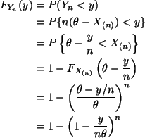
To apply the hint for part (a), we need to find the c. d. f. of Y_n
$$\begin{align*}F_{Y_n}(y) & = P(Y_n < y) \\ & = P\{ n (\theta - X_{(n)}) <... ...a} \right)^n \\ & = 1 - \left( 1 - \frac{y}{n \theta} \right)^n \end{align*}$$
Or, being more precise, using the fact that Y_n ranges from zero when $X_{(n)} = \theta$ to $n \theta$ when X_(n) = 0,

$$F_{Y_n}(y) = \begin{cases} 0, & y \le 0 \\ 1 - \left( 1... ...t)^n, & 0 < y < n \theta \\ 1, & y \ge n \theta \end{cases}$$

Now using the last part of the hint, this converges to

$$F_\infty(y) = \begin{cases} 0, & y \le 0 \\ 1 - e^{- y / \theta}, & 0 < y \end{cases}$$

and comparison with formula (2) on p. 166 in Lindgren shows this is indeed the c. d. f. of the $\text{Exp}(1 / \theta)$ distribution, so this shows

$$Y_n \stackrel{\mathcal{D}}{\longrightarrow}\text{Exp}(1 / \theta)$$

The Moral of the Story

Not all asymptotic distributions are normal. Not all asymptotics go at ``rate'' $\sqrt{n}$. Here we have

$$n (\theta - X_{(n)}) \stackrel{\mathcal{D}}{\longrightarrow}\text{Exp}(1 / \theta)$$

The asymptotic distribution is not normal, and the ``rate'' is nnot $\sqrt{n}$.

This is not the only example of ``nonstandard'' asymptotics. In fact, extreme values always have nonstandard asymptotics. The only reason for doing the $\mathcal{U}(0, \theta)$ case here is because the calculations are easiest for it.

N7-9

By Theorem 7.24 in the notes or Theorem 11 in Chapter 7 in Lindgren

$$Y = \frac{(n - 1) S^2_n}{\sigma^2}$$

is $\mathop{\rm chi}^2\nolimits(n - 1)$ distributed. Hence

$$P(S^2_n > 2 \sigma^2) = P\{Y > 2 (n - 1)\} = P(Y > 18)$$

Using Table Va in Lindgren, this is 0.035.

R gives the more precise answer

   > 1 - pchisq(18, 9)
   [1] 0.03517354

N7-10

(a)

Use Theorem 7 of Chapter 3 in Lindgren (the change-of-variable theorem in the special case of a linear transformation). This gives in the case $Y = \sigma X$

$$f_Y(y) = \frac{1}{\sigma} f_X(y / \sigma)$$

and using the functional form (2.42)
$$\begin{align*}f_Y(y) & = \frac{1}{\sigma} \cdot \frac{1}{\beta^\alpha \Gamma... ...a)^\alpha \Gamma(\alpha)} y^{\alpha - 1} e^{- y / (\sigma \beta)} \end{align*}$$
and this is clearly what we were to show.

(b)

One could argue as in part (a), but an even simpler way to do the problem is just to make the substitution $\beta = 1 / \lambda$in all the formulas of the problem. This obviously gives the desired result. You don't even have to write it out to see it.

N7-11

We are to calculate $E\{(Y - \mu_Y)^k\}$. Before we do that we need

$$\mu_Y = a + b \mu_X$$

(equation (1.14a) in the notes). Then
$$\begin{align*}E\{(Y - \mu_Y)^k\} & = E\{(a + b X - a - b \mu_X)^k\} \\ & = ... ... \\ & = E\{b^k (X - \mu_X)^k\} \\ & = b^k E\{(X - \mu_X)^k\} \end{align*}$$
by linearity of expectation. That's what was to be proved.

N7-12

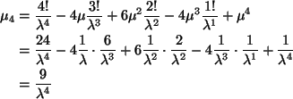
We need to calculate $\mu_2 = \sigma^2$ and $\mu_4$ for the $\mathop{\rm Exp}\nolimits(\lambda)$distribution. We know that $\sigma^2 = 1 / \lambda^2$. The fourth central moment is fairly obnoxious if done by hand
$$\begin{align*}\mu_4 & = E\{(X - \mu)^4\} \\ & = E(X^4 - 4 \mu X^3 + 6 \mu^... ... & = E(X^4) - 4 \mu E(X^3) + 6 \mu^2 E(X^2) - 4 \mu^3 E(X) + \mu^4 \end{align*}$$
by linearity of expectation. Now we can use the gamma integral

$$E(X^k) = \int_0^\infty x^k e^{- \lambda x} \, d x = \frac{\Gamma(k + 1)}{\lambda^k} = \frac{k !}{\lambda^k}$$

which can be looked up in the textbook as equation (4) on p. 173 in Lindgren or can be easily derived without looking it up by the trick of ``recognizing and unnormalized density,'' in this case a gamma density. Putting these two together gives
$$\begin{align*}\mu_4 & = \frac{4 !}{\lambda^4} - 4 \mu \frac{3 !}{\lambda^3} ... ...1}{\lambda^1} + \frac{1}{\lambda^4} \\ & = \frac{9}{\lambda^4} \end{align*}$$
The easy way is to feed it to Mathematica

In[1]:= f[x_] = lambda Exp[- lambda x]

         lambda
Out[1]= ---------
         lambda x
        E

In[2]:= mu = Integrate[ x f[x], {x, 0, Infinity},
        Assumptions -> {Re[lambda] > 0} ]

          1
Out[2]= ------
        lambda

In[4]:= mu4 = Integrate[ (x - mu)^4 f[x], {x, 0, Infinity},
        Assumptions -> {Re[lambda] > 0} ]

           9
Out[4]= -------
              4
        lambda

Either way we get

$$\mu_4 - \mu_2^2 = \frac{9}{\lambda^4} - \frac{1}{\lambda^4} = \frac{8}{\lambda^4}$$

and

$$V_n \approx \mathop{\mathcal{N}}\nolimits\left(\frac{1}{\lambda^2}, \frac{8}{n \lambda^4} \right).$$

The Moral of the Story

Note that here $\sigma = 1 / \lambda$so the asymptotic variance of the sample variance is $8 \sigma^4 / n$ here and $2 \sigma^4 / n$ in the normal case. Quite a difference.