Statistics 5101, Fall 2000, Geyer

Homework Solutions #11

Problem L7-1

(a)

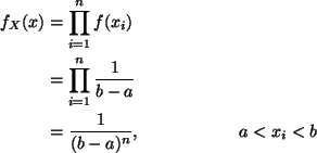
$$\begin{align*}f_X(x) & = \prod_{i=1}^n f(x_i) \\ & = \prod_{i=1}^n \frac{1}{b-a}\\ & = \frac{1}{(b - a)^n}, \hspace{2cm} a < x_i < b \end{align*}$$

(b)

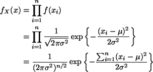
$$\begin{align*}f_X(x) & = \prod_{i=1}^n f(x_i) \\ & = \prod_{i=1}^n \frac{1}{ \... ...\left\{ - \frac{ \sum_{i=1}^n (x_i - \mu)^2} {2 \sigma^2} \right\} \end{align*}$$

(c)

$$\begin{align*}f_X(x) & = \prod_{i=1}^n f(x_i) \\ & = \prod_{i=1}^n p^{x_i} (1 ... ...{i = 1}^n x_i} (1 - p)^{n - \sum_{i=1}^n x_i}, \hspace{2cm} x_i=0,1 \end{align*}$$

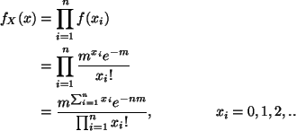
(d)

$$\begin{align*}f_X(x) & = \prod_{i=1}^n f(x_i) \\ & = \prod_{i=1}^n \frac{m^{x_... ..._i} e^{- nm}}{\prod_{i=1}^n x_i !}, \hspace{1.5cm} x_i = 0, 1,2, .. \end{align*}$$

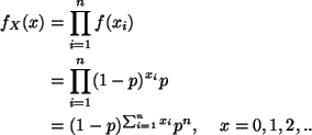
(e)

$$\begin{align*}f_X(x) & = \prod_{i=1}^n f(x_i) \\ & = \prod_{i=1}^n (1 - p)^{x_... ...\\ & = (1 - p)^{\sum_{i=1}^n x_i} p^n, \hspace{.4cm} x = 0,1,2,.. \end{align*}$$

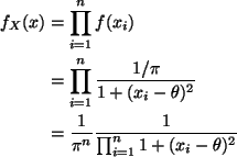
(f)

$$\begin{align*}f_X(x) & = \prod_{i=1}^n f(x_i) \\ & = \prod_{i=1}^n \frac{1/\pi... ...& = \frac{1}{\pi^n} \frac{1}{\prod_{i=1}^n 1+(x_{i}-\theta)^2} \\ \end{align*}$$

Problem L7-4

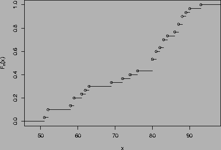
(a)

(b)

$$\begin{align*}X{\mkern -13.5 mu}\overline{\phantom{\text{X}}}& = \frac{1}{n} \sum_{i=1}^n X_i \\ & = \frac{2250}{30} \\ & = 75 \end{align*}$$

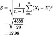
$$\begin{align*}S & = \sqrt{\frac{1}{n-1} \sum_{i=1}^n (X_i - X{\mkern -13.5 mu}\o... ...antom{\text{X}}})^2} \\ & = \sqrt{\frac{4888}{29}} \\ & = 12.98 \end{align*}$$

(c)

The two middle values (in sorted order) are both 80. Hence the median is 80.

(d)

There are n = 30 data points.

To find the p-th quantile of the empirical distribution, use Theorem 7.5 in the notes. For the lower quartile, p = 1 / 4. Then n p = 7.5 is not an integer, and the lower quartile is data point number $\lceil n p \rceil = 8$ (in sorted order), which is 62.

For the upper quartile, p = 3 / 4. Then n p = 22.5 is not an integer, and the lower quartile is data point number $\lceil n p \rceil = 23$ (in sorted order), which is 86.

(e)

The interquartile range is 86 - 62 = 24.

Problem L7-6

(a)

$$\sum X = n \times X{\mkern -13.5 mu}\overline{\phantom{\text{X}}}= 10 \times 5 = 50$$

$$\sum X^2 = n X{\mkern -13.5 mu}\overline{\phantom{\text{X}}}^2 + (n-1) S_X^2 = 10 \times 5^2 + 9 \times 2^2 = 286.$$

(b)

$$Y{\mkern -14.0 mu}\overline{\phantom{\text{Y}}}= 3 + 4 X{\mkern -13.5 mu}\overline{\phantom{\text{X}}}= 3 + 4 \times 5 = 23$$

$$S_Y = 4 S_X = 4 \times 2 = 8$$

Problem L7-13

$$X{\mkern -13.5 mu}\overline{\phantom{\text{X}}}\sim N(\mu, .16)$$

$$P(\lvert X{\mkern -13.5 mu}\overline{\phantom{\text{X}}}- \mu... ...ert > .8m) = P(\lvert Z \rvert > 2) = 2 \Phi(-2) = .0456$$

Problem L7-14

By the corollary on p. 210 in Lindgren we know that

$$E(S^2) = \sigma^2 = \frac{(1 - 0)^2}{12} = \frac{1}{12}.$$

In order to find the variance of S² we need to find $\mathop{\rm var}\nolimits(V)$using formula (5) p. 210 in Lindgren. Since

$$\mu_2 = \sigma^2_X = \frac{1}{12},$$

and

$$\mu_4 = \int_0^1 ( x - \frac{1}{2} )^4 \, d x = \frac{1}{80}$$

we have

$$\mathop{\rm var}\nolimits(V) = \frac{1}{180n} + \frac{1}{360n^2} - \frac{1}{120n^3}$$

and

$$\mathop{\rm var}\nolimits(S^2) = \frac{n^2}{(n - 1)^2} \matho... ...[ \frac{1}{180n} + \frac{1}{360n^2} - \frac{1}{120n^3} \right]$$

Sorry. The answer in the back of the book is wrong. It gives $\mathop{\rm var}\nolimits(V)$rather than $\mathop{\rm var}\nolimits(S^2)$.

Problem L7-16

(a)

$$E(D) = E( X{\mkern -13.5 mu}\overline{\phantom{\text{X}}}- Y{... ...Y{\mkern -14.0 mu}\overline{\phantom{\text{Y}}}) = 80 - 80 = 0$$

(b)

$$\mathop{\rm var}\nolimits(D) = \mathop{\rm var}\nolimits(X{\m... ... + \frac{\sigma^2}{n_Y} = \frac{36}{100} + \frac{36}{150} = .6$$

(c)

This cannot be done exactly, since the exact population distribution is not specified. By the central limit theorem $D \approx N( \mu_D, \sigma_D^2)$, that is, $D \approx N(0, .6)$. So we use that.
$$\begin{align*}P(\lvert D \rvert > 2) & = 1 - P( -2 < D < 2) \\ & = 1 - P( -2.582 < Z < 2.582)\\ & = 2 \Phi(-2.582) \\ & = 0.0098 \end{align*}$$

Problem L7-22

E(D) = 0

and

$$\mathop{\rm var}\nolimits(D) = 36 \left( \frac{1}{10} + \frac{1}{15} \right) = 6$$

So $D \sim N(0, 6)$, and
$$\begin{align*}P(\vert D\vert > 2) & = 1 - P( -2 < D < 2) \\ & = 1 - P(-0.8165 < Z < 0.8165)\\ & = 2 \Phi(-0.8165) \\ & = .414 \end{align*}$$

Problem L7-25

$$E \left( \frac{X{\mkern -13.5 mu}\overline{\phantom{\text{X}}... ...ht) E(X{\mkern -13.5 mu}\overline{\phantom{\text{X}}}_n - \mu)$$

by the independence of S_n and $X{\mkern -13.5 mu}\overline{\phantom{\text{X}}}_n$ (Corollary to Theorem 10 of Chapter 7 in Lindgren or Theorem 7.24 in the notes) assuming the expectations exist. We know the second expectation exists (because $X{\mkern -13.5 mu}\overline{\phantom{\text{X}}}_n$ is normal and the normal distribution has first moments) and is equal to zero because the first central moment is always zero (Theorem 2.9 in the notes).

Thus the expectation is zero if E(1 / S_n) exists. To prove that we need to look at the density of the gamma distribution of S_n², Equation (7.34) in the notes. Write Y_n = S²_n so

$$Y_n \sim \text{Gam}\left(\frac{n - 1}{2}, \frac{n - 1}{2 \sigma^2}\right)$$

Then $S_n = \sqrt{Y_n}$ so the existence question is: Does E(Y_n^{- 1/2})exist when Y_n has this gamma distribution? This existence problem was actually done as an example in the notes (Example 2.5.6). The result there is that if $X \sim \text{Gam}(\alpha, 1)$ then X^p has expectation whenever $p > - \alpha$. The same analysis applied here says that E(1 / S_n) exists if

$$p = - \frac{1}{2} > - \alpha = - \frac{n - 1}{2}$$

that is, if n > 2. So $E\left\{ (X{\mkern -13.5 mu}\overline{\phantom{\text{X}}}_n - \mu) / S_n \right\}$ is zero whenever n > 2 (and otherwise does not exist).

Problem N6-1

We need to show that if

$$Y_n = X_1 + X_2 + \ldots + X_n \sim \text{Cauchy}(n \mu, n \sigma)$$

then

$$\frac{1}{n} Y_n = X{\mkern -13.5 mu}\overline{\phantom{\text{X}}}_n \sim \text{Cauchy}(n \mu, n \sigma)$$

Thus this is simply a question about the linear change of variables

$$X{\mkern -13.5 mu}\overline{\phantom{\text{X}}}_n = \frac{1}{n} Y_n$$

The linear change of variable theorem (Theorem 7 of Chapter 3 in Lindgren) says

$\bar X_n = Y_n/n$, by the transformation theorem, the Jacobin J is n, and the density of $\bar X_n$ is

$$\begin{align*}f_{X{\mkern -13.5 mu}\overline{\phantom{\text{X}}}_n}(x) & = n f... ...+n^2[x - \mu]^2)} \\ & = \frac{\sigma}{\pi(\sigma^2+[x-\mu]^2)} \end{align*}$$
which is what was to be shown.

Problem N6-2

By the CLT

$$\sqrt{n} (\bar X_{n} - \mu) \stackrel{\mathcal{D}}{\longrightarrow}Y$$

where $Y \sim \mathcal{N}(0, \sigma^2)$. And by assumption

$$S_n \stackrel{P}{\longrightarrow}\sigma.$$

Put these together using Slutsky's theorem. The function

$$g(u, v) = \frac{u}{v}$$

is continuous except at v = 0 hence is continuous a every point of the form $(u, \sigma)$ because $\sigma > 0$ by assumption.

Hence

$$\frac{\sqrt{n} (\bar X_{n} - \mu)}{S_n} \stackrel{\mathcal{D}}{\longrightarrow}\frac{1}{\sigma} Y$$

and $Y / \sigma$ is standard normal by the rules for linear transformation of normal random variables.

Problem N6-3

The Y_n = I_A(X_n) are i. i. d. because functions of independent random variables are independent (Theorem 13 of Chapter 3 in Lindgren). The LLN says

$$Y{\mkern -14.0 mu}\overline{\phantom{\text{Y}}}_n \stackrel{P}{\longrightarrow}\mu_Y$$

so we only need to show that $\mu_Y = P(A)$, but this is obvious because ``probability is just expectation of indicator functions'' (Section 2.6 in the notes).

Problem N6-4

To do this problem, we need to recognize that the Y_n defined in the previous problem are $\text{Ber}(p)$ random variables. Every zero-one valued random variable X is Bernoulli with ``success'' probability p = P(X = 1). Every indicator function is zero-one valued, and P(I<sub>A</sub> = 1) = P(A) by definition (``probability is just expectation of indicator functions'' again).

Therefore
$$\begin{align*}E(Y_i) & = p \\ \mathop{\rm var}\nolimits(Y_i) & = p (1 - p) \end{align*}$$
and the LLN and CLT say

$$Y{\mkern -14.0 mu}\overline{\phantom{\text{Y}}}_n \stackrel{P}{\longrightarrow}p$$

and

$$\sqrt{n} (Y{\mkern -14.0 mu}\overline{\phantom{\text{Y}}}_n -... ...thcal{D}}{\longrightarrow}\mathcal{N}\bigl(0, p (1 - p) \bigr)$$

Now

$$g(u) = \sqrt{u (1 - u)}$$

is a continuous function, so the continuous mapping theorem applied to the LLN says

$$\sqrt{Y{\mkern -14.0 mu}\overline{\phantom{\text{Y}}}_n (1 - ... ...om{\text{Y}}}_n)} \stackrel{P}{\longrightarrow}\sqrt{p (1 - p}$$

if we call the left hand side S_n and the right hand side $\sigma$(it is the standard deviation of the Y_i), then apply Problem 6.2 to this statement and the CLT, we get what was to be shown.