next up previous
Up: Stat 5101 Homework Solutions

Statistics 5101, Fall 2000, Geyer


Homework Solutions #10

Problem L5-3

Let Yi = Xik, then Y1, Y2, $\ldots$ is a sequence of independent identically distributed random variables (functions of independent random variables are independent by Theorem 13 of Chapter 3 in Lindgren) with expectation

\begin{displaymath}\mu_Y = E(Y_i) = E(X^k).
\end{displaymath}

Then the LLN says

\begin{displaymath}Y{\mkern -14.0 mu}\overline{\phantom{\text{Y}}}_n \stackrel{P}{\longrightarrow}\mu_Y
\end{displaymath}

but this is just other notation for

\begin{displaymath}\frac{1}{n} \sum_{i = 1}^n X_i^k \stackrel{P}{\longrightarrow}E(X^k).
\end{displaymath}

Problem L5-6

Write Y for the weight of the 100 booklets. Then

\begin{displaymath}\begin{split}
E(Y) & = 100
\\
\mathop{\rm var}\nolimits(Y) & = 100 \times .02^2 = .04
\end{split}\end{displaymath}

so

\begin{displaymath}P(Y > 100.5)
=
1 - P(Y < 100.5)
=
1 - \Phi \left( \frac{1...
...100}{ \sqrt{100} \times .02} \right)
=
1 - \Phi(2.5) = .0062
\end{displaymath}

Problem L5-9

Let $Y \sim \mathcal{U}(-0.5, 0.5)$ be one error, then from the appendix on brand name distributions

\begin{displaymath}\begin{split}
E(Y) & = 0
\\
\mathop{\rm var}\nolimits(Y) & = \frac{1}{12}
\end{split}\end{displaymath}

If W is the sum of n i. i. d. such errors then

\begin{displaymath}\begin{split}
E(W) & = 0
\\
\mathop{\rm var}\nolimits(W) & = \frac{n}{12}
\end{split}\end{displaymath}

Thus

\begin{displaymath}\begin{split}
P\left(\lvert W \rvert < \sqrt{n}/2 \right)
&...
...\\
& = 1 - 2 \Phi(- \sqrt{3})
\\
& = 0.9167355
\end{split}\end{displaymath}

Problem L6-13

By direct count, the probability of a sum of 5 or less rolling a pair of dice is 5/18. Thus, if Y is the number of such rolls in 72 tries, $Y \sim \text{Bin}(72, 5/18)$, and

\begin{displaymath}\begin{split}
E(Y) & = 72 \times \frac{5}{18} = 20
\\
\ma...
...hop{\rm sd}\nolimits(Y) & = \sqrt{14.4444} = 3.8006
\end{split}\end{displaymath}

So, using a continuity correction,

\begin{displaymath}P(Y \ge 28) = 1 - \Phi \left( \frac{27 + 0.5 -
20}{3.8006} \right) = .0242
\end{displaymath}

Problem L6-86

From a picture of the triangular density, the two inside intervals have three times the probability of the outside intervals. Thus the probabilities of the intervals are $\frac{1}{8}$, $\frac{3}{8}$, $\frac{3}{8}$, and $\frac{1}{8}$.

Let X1, X2, X3, and X4 be the counts in the cells (1, 2, 2, 1), then this is a multinomial random vector and the probability of these counts is

\begin{displaymath}\begin{split}
\binom{n}{x_1, x_2, x_3, x_4} p_1^{x_1} p_2^{x...
...& =
180 \cdot \frac{3^4}{8^6}
\\
& =
0.0556183
\end{split}\end{displaymath}

Problem L12-12

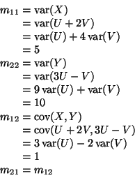
Since it is a linear transformation of a multivariate normal random vector, (X, Y) is also multivariate normal with mean vector zero because

\begin{displaymath}\begin{split}
E(X) & = E(U) + 2 E(V) = 0
\\
E(Y) & = 3 E(U) - E(V) = 0
\end{split}\end{displaymath}

and variance matrix M with components

\begin{displaymath}\begin{split}
m_{1 1}
& =
\mathop{\rm var}\nolimits(X)
\\...
...olimits(V)
\\
& =
1
\\
m_{2 1}
& =
m_{1 2}
\end{split}\end{displaymath}

Problem N5-7

From the variance formula for the multinomial in the appendix on brand name distributions

\begin{displaymath}\begin{split}
\mathop{\rm var}\nolimits(X_i - X_j)
& =
\ma...
... p_i p_j
\\
& =
n [ p_i + p_j - (p_i - p_j)^2 ]
\end{split}\end{displaymath}

Problem N5-10

The problem is to specialize the formula
\begin{displaymath}f_{\mathbf{X}}(\mathbf{x})
=
\frac{1}{(2 \pi)^{n / 2} \det(...
...{\mu})' \mathbf{M}^{-1} (\mathbf{x}- \boldsymbol{\mu}) \right)
\end{displaymath}

for the density of the multivariate normal to the two-dimensional case, when the mean vector is

\begin{displaymath}\boldsymbol{\mu}= \begin{pmatrix}\mu_X \\ \mu_Y \end{pmatrix}\end{displaymath}

and the variance matrix is

\begin{displaymath}\mathbf{M}= \begin{pmatrix}\sigma^2_X & \rho \sigma_X \sigma_Y \\
\rho \sigma_X \sigma_Y & \sigma^2_Y \end{pmatrix}\end{displaymath}

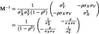
Using the hints

\begin{displaymath}\det(\mathbf{M}) = \sigma^2_X \sigma^2_Y (1 - \rho^2)
\end{displaymath}

and

\begin{displaymath}\renewcommand{\arraystretch}{1.25}
\begin{split}
\mathbf{M}^...
...gma_X \sigma_Y} & \frac{1}{\sigma^2_Y} \end{pmatrix}\end{split}\end{displaymath}

The constant part of the density is now done

\begin{displaymath}\frac{1}{(2 \pi)^{n / 2} \det(\mathbf{M})^{1 / 2}}
=
\frac{1}{2 \pi \sigma_X \sigma_Y \sqrt{1 - \rho^2}}
\end{displaymath}

because n = 2. So the only thing left is to match up the quadratic form in the exponent.

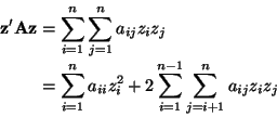
In general a quadratic form is written out explicitly in terms of components as
\begin{displaymath}\begin{split}
\mathbf{z}' \mathbf{A}\mathbf{z}
& =
\sum_{i...
...i = 1}^{n - 1}
\sum_{j = i + 1}^n
a_{i j} z_i z_j
\end{split}\end{displaymath}

In this case the quadratic form in the exponent is
\begin{multline*}(\mathbf{x}- \boldsymbol{\mu})' \mathbf{M}^{-1} (\mathbf{x}- \b...
... \frac{\rho (x - \mu_X) (y - \mu_Y)}{\sigma_X \sigma_Y}
\right)
\end{multline*}
which is the quadratic form in the formula to be proved. So we're done.

Problem N5-11

In this case the elements of the partitioned variance matrix are all scalars
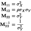
\begin{displaymath}\begin{split}
\mathbf{M}_{1 1} & = \sigma^2_X
\\
\mathbf{...
...\\
\mathbf{M}_{2 2}^{-1} & = \frac{1}{\sigma^2_Y}
\end{split}\end{displaymath}

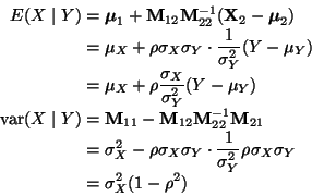
Hence

\begin{displaymath}\begin{split}
E(X \mid Y)
& =
\boldsymbol{\mu}_1 + \mathbf...
...sigma_X \sigma_Y
\\
& =
\sigma^2_X (1 - \rho^2)
\end{split}\end{displaymath}

Problem N5-12

We are to calculate $P\{ q(\mathbf{X}) < d \}$ for given d, where

\begin{displaymath}q(\mathbf{x})
=
(\mathbf{x}- \boldsymbol{\mu})' \mathbf{M}^{-1} (\mathbf{x}- \boldsymbol{\mu})
\end{displaymath}

and

\begin{displaymath}\mathbf{X}\sim \mathcal{N}(\boldsymbol{\mu}, \mathbf{M})
\end{displaymath}

Now Problem 12-32 in Lindgren referred to in the hint says almost the same what we want

\begin{displaymath}q_2(\mathbf{Y}) = \mathbf{Y}' \mathbf{M}^{-1} \mathbf{Y}\sim \text{chi}^2(p)
\end{displaymath}

where

\begin{displaymath}\mathbf{Y}\sim \mathcal{N}(0, \mathbf{M})
\end{displaymath}

The only differences are (1) we have no means subtracted off in q2and (2) Y has mean zero. However,

\begin{displaymath}q(\mathbf{X}) = q_2(\mathbf{X}- \boldsymbol{\mu})
\end{displaymath}

and

\begin{displaymath}\mathbf{X}- \boldsymbol{\mu}\sim \mathcal{N}(0, \mathbf{M})
\end{displaymath}

so we can apply the 12-32 to this problem obtaining

\begin{displaymath}q(\mathbf{X}) \sim \text{chi}^2(p)
\end{displaymath}

Thus

\begin{displaymath}P\{ q(\mathbf{X}) < d \} = F(d),
\end{displaymath}

where F is the the c. d. f. of the $\text{chi}^2(p)$ distribution.

Problem N5-13

(a)

Write

\begin{displaymath}\mathbf{Z}= \begin{pmatrix}U - V \\ V - W \end{pmatrix}\end{displaymath}

Then

\begin{displaymath}\mathbf{Z}
=
\begin{pmatrix}1 & -1 & 0 \\ 0 & 1 & -1 \end{pmatrix} \begin{pmatrix}U \\ V \\ W \end{pmatrix}\end{displaymath}

thus is a linear transformation of multivariate normal, hence multivariate normal with

\begin{displaymath}E(\mathbf{Z})
=
\begin{pmatrix}1 & -1 & 0 \\ 0 & 1 & -1 \en...
... \\ 0 \\ 0 \end{pmatrix} =
\begin{pmatrix}0 \\ 0 \end{pmatrix}\end{displaymath}

and

\begin{displaymath}\mathop{\rm var}\nolimits(\mathbf{Z})
=
\begin{pmatrix}1 & ...
... \end{pmatrix} =
\begin{pmatrix}2 & -1 \\ -1 & 2 \end{pmatrix}\end{displaymath}

(b)

From the formula for the variance,

\begin{displaymath}\mathop{\rm var}\nolimits(Z_1) = \mathop{\rm var}\nolimits(Z_2) = 2
\end{displaymath}

and

\begin{displaymath}\mathop{\rm cor}\nolimits(Z_1, Z_2) = - \frac{1}{2}
\end{displaymath}

Thus the conditional distribution of Z1 given Z2is normal with mean

\begin{displaymath}E(Z_1 \mid Z_2)
=
- \frac{1}{2} \cdot Z_2
\end{displaymath}

and variance

\begin{displaymath}\mathop{\rm var}\nolimits(Z_1 \mid Z_2)
=
2 \left[1 - \left(- \frac{1}{2}\right)^2 \right]
=
\frac{3}{2}
\end{displaymath}


next up previous
Up: Stat 5101 Homework Solutions
Charles Geyer
2000-12-13