Statistics 5101, Fall 2000, Geyer

Homework Solutions #9

Problem L12-32

A general normal random variable X has the form X= a+ BZ, where $\mathbf{Z}\sim \mathcal{N}(0, \mathbf{I})$. In order for X to have mean zero, we need a= 0. Thus X= BZ, and in order for X to be nondegenerate, B must be invertible, in which case

$$\mathbf{M}= \mathop{\rm var}\nolimits(\mathbf{X}) = \mathbf{B}\mathbf{B}'$$

and

M^-1 = (B')^-1 B^-1

and

Q = X' M^-1 X = X' (B')^-1 B^-1 X = Z' Z

because Z= B^-1 X. Now

$$\mathbf{Z}' \mathbf{Z}= \sum_{i = 1}^p Z_i^2$$

is the sum of squares of p independent standard normal random variables, hence $\text{chi}^2(p)$ distributed.

Problem N5-1

Using R for the computer work

> M <- matrix(c(3, 2, -1, 2, 3, 2, -1, 2, 3), nrow=3)
> M
     [,1] [,2] [,3]
[1,]    3    2   -1
[2,]    2    3    2
[3,]   -1    2    3
> eigen(M)
$values
[1]  5.3722813  4.0000000 -0.3722813

$vectors
          [,1]          [,2]       [,3]
[1,] 0.4544013 -7.071068e-01 -0.5417743
[2,] 0.7661846 -1.155753e-16  0.6426206
[3,] 0.4544013  7.071068e-01 -0.5417743

The negative eigenvalue -0.3722813 means this is not a positive semi-definite matrix, hence not a variance matrix.

Problem N5-2

Using R for the computer work

> M <- matrix(c(3, 2, -1/3, 2, 3, 2, -1/3, 2, 3), nrow=3)
> M
           [,1] [,2]       [,3]
[1,]  3.0000000    2 -0.3333333
[2,]  2.0000000    3  2.0000000
[3,] -0.3333333    2  3.0000000
> eigen(M)
$values
[1] 5.666667 3.333333 0.000000

$vectors
          [,1]          [,2]       [,3]
[1,] 0.4850713 -7.071068e-01 -0.5144958
[2,] 0.7276069 -2.473336e-19  0.6859943
[3,] 0.4850713  7.071068e-01 -0.5144958

Since all three eigenvalues are nonnegative, this is a possible covariance matrix, but since one of the eigenvalues is zero, M is not positive definite and the random variable is degenerate.

Problem N5-3

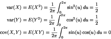
The only hard thing about this problem is realizing it is simple (and perhaps looking up how to integrate trig functions).

$$\begin{split} E(X) & = \frac{1}{2 \pi} \int_0^{2 \pi} \... ...{1}{2 \pi} \int_0^{2 \pi} \cos(u) \, d u = 0 \end{split}$$

Hence the mean vector is zero. Then

$$\begin{split} \mathop{\rm var}\nolimits(X) & = E(X^2)... ...} \int_0^{2 \pi} \sin(u) \cos(u) \, d u = 0 \end{split}$$

So

$$\mathop{\rm var}\nolimits\left\{ \begin{pmatrix}X \\ Y \end{p... ...egin{pmatrix}\frac{1}{2} & 0 \\ 0 & \frac{1}{2} \end{pmatrix}$$

Interesting Comment

Not part of the problem, but we have here another example that uncorrelated does not imply independent. $\mathop{\rm cov}\nolimits(X, Y) = 0$, but having a degenerate joint distribution, X and Y are highly dependent. Indeed, since the vector (X, Y) is concentrated on the unit circle, X² + Y² = 1 with probability one (essentially because of the trig identity $\sin^2 u + \cos^2 u = 1$ for all u). Thus the conditional distribution of Y given X is concentrated at the two points $\pm \sqrt{1 - X^2}$. So X almost determines Y (it determines the absolute value, only the sign is still random).

Problem N5-4

In general

$$\mathbf{w}' \mathbf{M}\mathbf{w} = \sum_{k = 1}^n \sum_{l = 1}^n m_{k l} w_k w_l$$

If we choose w so that only w_i and w_j are nonzero, this becomes

m_{i i} w_i² + 2 m_{i j} w_i w_j + m_{j j} w_j²

and this must be nonnegative for any choice of w_i and w_j

$$m_{i i} w_i^2 + 2 m_{i j} w_i w_j + m_{j j} w_j^2 \ge 0$$ (1)

Try

$$\begin{split} w_i & = 1 / \sqrt{m_{i i}} \\ w_j & = 1 / \sqrt{m_{j j}} \end{split}$$

Then (1) becomes

$$1 + 2 \frac{m_{i j}}{\sqrt{m_{i i} m_{j j}}} + 1 \ge 0$$

which implies one of the inequalities to be proved. If instead make w_j negative, we get the same thing with a minus sign on the middle term, and that proves the other inequality.

Problem N5-5

If the dimension is n = 1, then the variance matrix is just a scalar $\mathbf{M}= \sigma^2$ and $\mathbf{M}^{-1} = 1 / \sigma^2$ and $\det{\mathbf{M}} = \sigma^2$. Making all these changes turns (5.24) on p. 144 of the notes into (9) on p. 180 in Lindgren.

Problem N5-6

A vector X concentrated at the point a has

$$\begin{split} E(\mathbf{X}) & = \mathbf{a} \\ \mathop{\rm var}\nolimits(\mathbf{X}) & = 0 \end{split}$$

(the variance matrix being the zero matrix). Our definition of multivariate normal says there is a multivariate normal random vector with this mean and variance, namely the vector Y= a+ BZ, where Z is a standard multivariate normal random vector and we choose B to also be the zero matrix. Clearly Y is also concentrated at a and thus is equal to X with probability one.

Problem N5-8

Any linear transformation of multivariate normal is again multivariate normal (Theorem 12 of Chapter 12 in Lindgren, inexplicably omitted from the notes). Thus Y is multivariate normal. Hence to figure out which normal, we only need to find its parameters (mean vector and variance matrix).

$$\begin{split} E(\mathbf{Y}) & = \mathbf{M}^{-1} E(\mathbf{X... ...1} \mathbf{M}\mathbf{M}^{-1} = \mathbf{M}^{-1} \end{split}$$

Thus $\mathbf{Y}\sim \mathcal{N}(0, \mathbf{M}^{-1})$.