Up: Stat 5101 Homework Solutions
Statistics 5101, Fall 2000, Geyer
Homework Solutions #8
We have a Poisson process with an average interarrival time of two minutes
(i. e.  ), and rate parameter
 (per min.).
Waiting times are
(per min.).
Waiting times are
 distributed, so
that six minutes will elapse with no customer arrivals is
distributed, so
that six minutes will elapse with no customer arrivals is
Since the arrival process is Poisson,
Since the exponential distribution is ``memoryless'':
The waiting time until the third customer arrival has
a
 distribution,
so the expected value is
distribution,
so the expected value is
 .
It is the same as average time to the next.
The time to the third failure after any point in time is
.
It is the same as average time to the next.
The time to the third failure after any point in time is
 .
Then the mean
time to the third failure is
.
Then the mean
time to the third failure is
 days.
The expected number of failures in 10 days is
days.
The expected number of failures in 10 days is
 .
.
So the distribution of the time to failure of the system
is Exp(0.8).
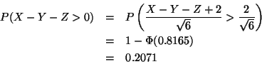
Using formula (11) page 181 in Lindgren
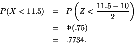
The quartiles of the standard normal distribution are  (or perhaps 0.675, hard to tell) from Table I in Lindgren (p. 576).
R says
(or perhaps 0.675, hard to tell) from Table I in Lindgren (p. 576).
R says
> qnorm(0.25)
[1] -0.6744898
The quartiles of a
 random variable are
 or 8.65 and 11.35.
This whole problem can be done in one step by computer
or 8.65 and 11.35.
This whole problem can be done in one step by computer
> qnorm(0.25, 10, 2)
[1] 8.65102
> qnorm(0.75, 10, 2)
[1] 11.34898
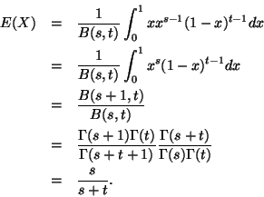
The mapping
 is two-to-one,
so we need to use Theorem 1.8 in the notes.
The mapping has two right inverses
h+(y) = x and
h-(y) = - x.
The derivatives are
is two-to-one,
so we need to use Theorem 1.8 in the notes.
The mapping has two right inverses
h+(y) = x and
h-(y) = - x.
The derivatives are  ,
so the absolute values of the derivatives
ignored. Thus,
,
so the absolute values of the derivatives
ignored. Thus,
Since the density fX is symmetric,
fY(y) = 2 fX(y).
Thus
and
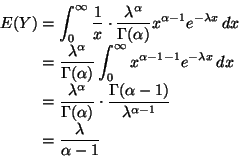
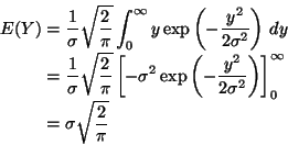
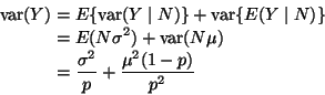
Since
 ,
,
and
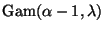
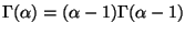
because the second parameter of the gamma is a scale parameter
by Theorem 7 of Chapter 3 in Lindgren. Doing the plug-in indeed shows
 .
.
and
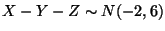
Write
 and
and
 so
so
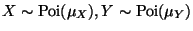 .
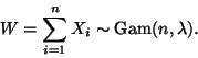
Since X and Y are independent,
.
Since X and Y are independent,
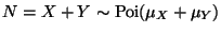 (marginally).
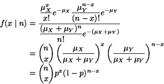
Now we need to know the joint distribution of X and N to calculate the
conditional, but we aren't given that. What we can easily do is the joint
of X and Y
(marginally).
Now we need to know the joint distribution of X and N to calculate the
conditional, but we aren't given that. What we can easily do is the joint
of X and Y
Now we do a change of variables. There is no Jacobian for discrete, change
of variables, but otherwise much the same plug in y as a function of the
new variables, that is, y = n - x, obtaining
Now the conditional is joint over marginal
if we define
If you didn't try this, ignore this answer. This is just for the people
who struggled with this failed problem and want to know what the actual
answer was. It is actually fairly obvious when looked at the right way
(which the author of the question, Geyer, obviously didn't when writing it).
Since X is independent of Y the distribution of Y given X is the
same as the marginal distribution of Y
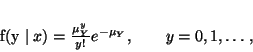 |
(1) |
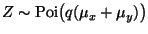
and the distribution of N = X + Y
given X is the same as the distribution of a constant plus a Poisson:
X is constant when conditioning on it and Y is Poisson. Thus
we get the density of N given X by plugging y = n - x into (1)
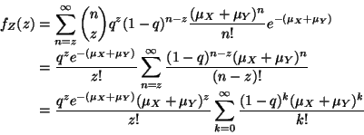
The joint distribution of Z and N is
We find the marginal of Z by summing out N
Now the sum is almost the integral of
a
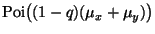 density. It only needs the
exponential factor for that density
density. It only needs the
exponential factor for that density
Hence
 .
Logically part (a) comes first, but it is a bit easier to see what's going
on if we do part (b) first, remembering that we're not sure yet whether
the integral exists.
If the integral exists
.
Logically part (a) comes first, but it is a bit easier to see what's going
on if we do part (b) first, remembering that we're not sure yet whether
the integral exists.
If the integral exists
where we did the integral by recognizing the integrand is an unnormalized
 density and simplified the ratio of
gamma functions using
the recursion formula
density and simplified the ratio of
gamma functions using
the recursion formula
 .
Note that the integral is clearly bogus if
.
Note that the integral is clearly bogus if
 ,
because then
,
because then
 is not defined. Also the last line gives zero or
a negative number for the expectation of a positive random variable when
.
So presumably the problem in part (a) is to rule out
and perhaps other parameter values. We'll see.
Constants are irrelevant, the question is for what values of
is not defined. Also the last line gives zero or
a negative number for the expectation of a positive random variable when
.
So presumably the problem in part (a) is to rule out
and perhaps other parameter values. We'll see.
Constants are irrelevant, the question is for what values of  and
and
 (with
(with
 and
and
 already required just by
definition of the gamma distribution) does the integral
already required just by
definition of the gamma distribution) does the integral
exist. There are two things to check
- near infinity
- singularities
By Lemma 2.41 in the notes, or just by the fact that
 goes
to zero as x goes to infinity faster than any power of x, there is no
problem near infinity.
Thus the only problem is near zero, where the integrand behaves
like
goes
to zero as x goes to infinity faster than any power of x, there is no
problem near infinity.
Thus the only problem is near zero, where the integrand behaves
like
 and has a singularity if
 .
But
Lemma 2.40 in the notes says the singularity if integrable if the exponent
is greater than - 1, that is if
.
But
Lemma 2.40 in the notes says the singularity if integrable if the exponent
is greater than - 1, that is if
 .
So that's the condition:
and
.
Since
.
So that's the condition:
and
.
Since
 ,
,
Up: Stat 5101 Homework Solutions
Charles Geyer
2000-11-14
![\begin{eqnarray*}P(X \leq 2) & = & \sum_{k=0}^2 \frac{e^{- \lambda t} (\lambda t...
... = & e^{- 3} \left[ 1 + 3 + \frac{9}{2} \right] \\
& = & .423
\end{eqnarray*}](img5.gif)
![\begin{eqnarray*}P(X \leq 3) & = & \sum_{k=0}^3 \frac{e^{- \lambda t} (\lambda t...
...+ \frac{(2.8)^2}{2} + \frac{(2.8)^3}{6} \right] \\
& = & .692
\end{eqnarray*}](img13.gif)
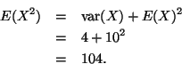
![\begin{eqnarray*}E[(X - 10)^4] & = & \sigma^4 E(Z^4) \\
& = & (2 \times 2 - 1) (2 \times 2 - 3) \sigma^4 \\
& = & 48.
\end{eqnarray*}](img19.gif)
![\begin{eqnarray*}E(X^3) & = & E \left[ [(X - 10) + 10]^3 \right] \\
& = & E[(X...
...+ 10^3 \\
& = & 0 + 30 \sigma^2_X + 0 + 1000 \\
& = & 1120.
\end{eqnarray*}](img20.gif)
![\begin{displaymath}\begin{split}
f_Z(z)
& =
\frac{q^z e^{- (\mu_X + \mu_Y)...
...(\mu_X + \mu_Y)]^z}{z !} e^{- q (\mu_X + \mu_Y)}
\end{split}
\end{displaymath}](img50.gif)