next up previous
Up: Stat 5101 Homework Solutions

Statistics 5101, Fall 2000, Geyer


Homework Solutions #6

Problem L3-43

(a)

The joint density function of X and Y, is

\begin{displaymath}f(x, y) = 2, \qquad 0 < x,\ 0 < y, x + y < 1.
\end{displaymath}

The marginal density for X is then

\begin{displaymath}f_X(x) = \int_0^{1 - x} 2 \, d y = 2 (1 - x), \qquad 0 < x < 1,
\end{displaymath}

and by symmetry Y has the same marginal (same as a function, not same as a formula)

\begin{displaymath}f_Y(y) = 2 (1 - y), \qquad 0 < y < 1.
\end{displaymath}

(b)

One conditional density function is

\begin{displaymath}f(x \mid y) = \frac{f(x, y)}{f_Y(y)} = \frac{1}{1 - y},
\qquad 0 < x < 1 - y,\ 0 < y < 1
\end{displaymath}

and, by symmetry, the other is the same formula with x and y interchanged.

Problem L4-10

Since X and Y are independent,

\begin{displaymath}E(X \mid Y) = E(X) = \int_0^\infty x f(x) \, d x = \int_0^\infty x e^{-x} \,
d x = 1.
\end{displaymath}

Problem L4-20

(a)

By Theorem 10 (p. 72) in Lindgren and also by the section on ``conditional probability as renormalization'' in the notes, the conditional distributions of a uniform distribution are uniform. Hence $X \mid Y \sim \mathcal{U}(0, y)$, and the mean of this distribution is $E(X \mid y) = y / 2$.

(b)


\begin{displaymath}E(X) = E\{E(X \mid Y)\} = E(Y / 2) = E(Y) / 2
\end{displaymath}

(c)

Nothing easy here, have to just do it,

\begin{displaymath}\begin{split}
E\{(Y - X)^2\}
& =
\int_0^1 \int_0^y (y - x)...
...t[ \frac{y^4}{4} \right]_0^1
\\
& =
\frac{1}{6}
\end{split}\end{displaymath}

Problem L4-55


\begin{displaymath}\begin{split}
\psi(t) & = (1 - t^2)^{-1}
\\
\psi'(t) & = ...
...2}
\\
\psi''(t) & = 2 (1 + 3 t^2) (1 - t^2)^{-3}
\end{split}\end{displaymath}

So

\begin{displaymath}\begin{split}
E(X) = \psi'(0) & = 0
\\
E(X^2) = \psi''(0) & = 2
\end{split}\end{displaymath}

and

\begin{displaymath}\mathop{\rm var}\nolimits(X) = E(X^2) - E(X)^2 = 2.
\end{displaymath}

Problem L4-58

If

\begin{displaymath}h(x) = e^{- x^2 / 2}, \qquad - \infty < x < + \infty
\end{displaymath}

is an unnormalized density, then the normalized density is

\begin{displaymath}f(x) = \frac{1}{c} e^{- x^2 / 2}, \qquad - \infty < x < + \infty
\end{displaymath}

where

 \begin{displaymath}
c = \int_{-\infty}^\infty e^{- x^2 / 2} \, d x.
\end{displaymath} (1)

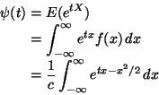
The m. g. f. is

\begin{displaymath}\begin{split}
\psi(t)
& =
E(e^{t X})
\\
& =
\int_{-\in...
...}{c} \int_{-\infty}^\infty e^{t x - x^2 / 2} \, d x
\end{split}\end{displaymath}

at present we don't know how to do this integral unless we can somehow put it in the form of (1). So that's what we try.

First we ``complete the square'' in the exponent

\begin{displaymath}t x - \frac{x^2}{2} = - \frac{(x - t)^2}{2} + \frac{t^2}{2}
\end{displaymath}

So

\begin{displaymath}\psi(t)
=
\frac{e^{t^2 / 2}}{c} \int_{-\infty}^\infty e^{- (x - t)^2 / 2} \, d x
\end{displaymath}

Now the integral can be evaluated using the substitution s = x - t

\begin{displaymath}\int_{-\infty}^\infty e^{- (x - t)^2 / 2} \, d x
c
\int_{-\infty}^\infty e^{- s^2 / 2} \, d s
=
c
\end{displaymath}

Thus finally,

\begin{displaymath}\psi(t) = e^{t^2 / 2}
\end{displaymath}

Problem N2-35

(a)

From (2.61), the marginal density of X is

\begin{displaymath}f_X(x) = \int_0^1 f(x, y) \, d y = \int_0^1 4 x y \, d y = 2 x.
\end{displaymath}

Because this problem is symmetric under the interchange of x and y, the marginal density of Y is the same function fY(y) = 2 y.

Now since,

f(x, y) = fX(x) fY(y)

this satisfies the factorization criterion.

(b)

In (2.62) the domains of integration depend on the other variable. The marginal density of X is

\begin{displaymath}f_X(x)
=
\int_x^1 f(x, y) \, d y
=
\int_x^1 8 x y \, d y
...
...4 x y^2 \biggl\vert _x^1
=
4 x (1 - x)^2,
\qquad 0 < x < 1.
\end{displaymath}

And the marginal density of Y is

\begin{displaymath}f_Y(y)
=
\int_0^y f(x, y) \, d x
=
\int_0^y 8 x y \, d x
=
4 x^2 y \biggl\vert _0^y
=
4 y^3
\qquad 0 < y < 1.
\end{displaymath}

And the factorization criterion is not satisfied.

Problem N2-36

By the definition of independence, equation (2.58) in the notes, E(X Y) = E(X) E(Y). Hence

\begin{displaymath}\mathop{\rm cov}\nolimits(X, Y) = E(X Y) - E(X) E(Y) = 0.
\end{displaymath}

Problem N2-37

(a)

E(X) = 0 because X is symmetric about 0, and E(X Y) = E(X3) = 0. By the symmetry of X and Theorem 2.10. Thus

\begin{displaymath}\mathop{\rm cov}\nolimits(X, Y) = E(X Y) - E(X) E(Y) = 0.
\end{displaymath}

(b)

As the hint says, there exists an event A such that $0 < P(X \in A) < 1$. If X were independent of itself, then we would have

\begin{displaymath}P(X \in A) = P(X \in A \mathop{\rm and}\nolimits X \in A) = P(X \in A)^2
\end{displaymath}

and this is impossible. The only numbers that are their own squares are zero and one, and we have disallowed those values for $P(X \in A)$.

Problem N2-38

First note that $E(X) = \mu = \alpha_1$, just by definition of these notations. Then
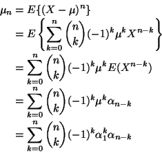
\begin{displaymath}\begin{split}
\mu_n
& =
E\{(X - \mu)^n\}
\\
& =
E\left...
... 0}^n \binom{n}{k} (-1)^{k} \alpha_1^k \alpha_{n-k}
\end{split}\end{displaymath}

where the second equality is the binomial theorem, the third is linearity of expectation, and the last is just $\mu = \alpha_1$.

To apply the same trick to $\alpha_n = E(X^n)$, we first need to express X as a binomial, and, in order to eventually produce $\mu_{n - k}$ terms, the binomial must involve $(X - \mu)$, thus the obvious expression

\begin{displaymath}X = (X - \mu) + \mu.
\end{displaymath}

Then

\begin{displaymath}\begin{split}
\alpha_n
& =
E\{[(X - \mu) + \mu]^n\}
\\
...
...=
\sum_{k = 0}^n \binom{n}{k} \alpha_1^k \mu_{n-k}
\end{split}\end{displaymath}

Problem N3-1


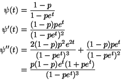
\begin{displaymath}\begin{split}
\psi(t) & = \frac{1 - p}{1 - p e^t}
\\
\psi...
... =
\frac{p (1 - p) e^t (1 + p e^t)}{(1 - p e^t)^3}
\end{split}\end{displaymath}

So

\begin{displaymath}\begin{split}
E(X) = \psi'(0) & = \frac{p}{1 - p}
\\
E(X^2) = \psi''(0)
& =
\frac{p (1 + p)}{(1 - p)^2}
\end{split}\end{displaymath}

and

\begin{displaymath}\mathop{\rm var}\nolimits(X)
=
E(X^2) - E(X)^2
=
\frac{p + p^2}{(1 - p)^2} - \frac{p^2}{(1 - p)^2}
=
\frac{p}{(1 - p)^2}
\end{displaymath}

Problem N3-2


\begin{displaymath}E(Y \mid x) = \int_{0}^{1 - x} y f(y \mid x) \, d y
= \frac{1}{1-x} \int_0^{1 - x} y \, d y =
\frac{1-x}{2}
\end{displaymath}


\begin{displaymath}E(Y^2 \mid x) = \int_0^{1 - x} y^2 f(y \mid x) \, d y
= \frac{1}{1-x} \int_0^{1 - x} y^2 \, d y =
\frac{(1-x)^2}{3}
\end{displaymath}

So

\begin{displaymath}\mathop{\rm var}\nolimits(Y \mid x) = E(Y^2 \mid x) - E(Y \mid x)^2 = \frac{(1 - x)^2}{12}
\end{displaymath}

Problem N3-3

(a)


\begin{displaymath}E(Y \mid x)
=
\int_0^x y f(y \mid x) \, d y
=
\int_0^x \frac{2 y^2}{x^2} \, d y
=
\frac{2x}{3}
\end{displaymath}

and

\begin{displaymath}E(Y^2 \mid x)
=
\int_0^x y^2 f(y \mid x) \, d y
=
\int_0^x \frac{2 y^3}{x^2} \, d y
=
\frac{x^2}{2}
\end{displaymath}

so

\begin{displaymath}\mathop{\rm var}\nolimits(Y \mid x)
=
E(Y^2 \mid x) - E(Y \mid x)^2
=
\frac{x^{2}}{18}
\end{displaymath}

Problem N3-4

If the integral exists, the function is

\begin{displaymath}c(\theta) = \int_0^1 x^\theta \, d x = \frac{1}{\theta + 1}
\end{displaymath}

From Lemma 2.40 in the notes we know the integral exists if and only if the exponent is greater than - 1, hence

\begin{displaymath}c(\theta) = \frac{1}{\theta + 1}, \qquad \theta > - 1.
\end{displaymath}

Note: The formula for $c(\theta)$ produces a completely ridiculous result when $\theta < - 1$, saying that the integral of a positive function is negative. Thus it is important to check whether integrals exist. The formalism of doing the indefinite integral and plugging in the limits won't tell when what you are doing is completely wrong!

Problem N3-5


\begin{displaymath}E(X) = E\{ E(X \mid Y, Z) \} = E(Y)
\end{displaymath}

and

\begin{displaymath}\mathop{\rm var}\nolimits(X) = E\{ \mathop{\rm var}\nolimits(...
...its\{ E(X \mid Y, Z) \}
= E(Z) + \mathop{\rm var}\nolimits(Y)
\end{displaymath}

Problem N3-6

The joint density is

\begin{displaymath}f(x, y) = \frac{1}{4 \pi}, \qquad x^ + y^2 < 4
\end{displaymath}

since the area of the domain is $4 \pi$.

(a)

By the principle that the conditionals of a uniform are uniform, this is some one-dimensional uniform distribution. The only issue is to figure out the ranges. The range of x when y is fixed consists of the x such that x2 + y2 < 4, which is

\begin{displaymath}- \sqrt{4 - y^2} < x < \sqrt{4 - y^2}
\end{displaymath}

Thus

\begin{displaymath}X \mid Y \sim \mathcal{U}(- \sqrt{4 - y^2}, \sqrt{4 - y^2})
\end{displaymath}

and this distribution has density

\begin{displaymath}f(x \mid y) = \frac{1}{2 \sqrt{4 - y^2}}, \qquad
\lvert x \rvert < \sqrt{4 - y^2}
\end{displaymath}

Because the problem is symmetric under the interchange of X and Y, the other conditional can be found by interchanging x and y in the formula.

(b)

Since $\text{marginal} = \text{joint} / \text{conditional}$,

\begin{displaymath}f_Y(y) = \frac{f(x, y)}{f(x \mid y)}
=
\frac{1 / 4 \pi}{1 /...
...t{4 - y^2}}
=
\frac{\sqrt{4 - y^2}}{2 \pi}, qquad -2 < y < 2
\end{displaymath}

and the marginal of X is the same with y's replaced by x's.

(c)

From part(a), the distribution of $Y \mid X$ is symmetric about zero, so has mean zero.

(d)

This is tricky because it involves case splitting. For x near $\pm 2$, the entire range of the distribution of $Y \mid X$lies between + 1 and - 1. Hence in this case $P(\lvert Y \rvert < 1 \mid x) = 1$.

For x near 0, the interval (-1, 1) is a proper subinterval of the range of $Y \mid X$, and the probability is the area under the density over this interval, which is just base times height (the area of a rectangle). Hence in this case

\begin{displaymath}P(\lvert Y \rvert < 1 \mid x) = [1 - (-1)] \times \frac{1}{2 \sqrt{4 - x^2}}
=
\frac{1}{\sqrt{4 - x^2}}
\end{displaymath}

The only thing left is to find the x where the two cases split. That is where the range of $Y \mid X$ is exactly (-1, 1), that is, where

\begin{displaymath}1 = \sqrt{4 - x^2}
\end{displaymath}

or x2 = 3 or $x = \pm \sqrt{3}$. Putting everything together

\begin{displaymath}P(\lvert Y \rvert < 1 \mid x)
=
\begin{cases}
\frac{1}{\sq...
... x^2 < 4 \\
\text{arbitrary}, & \text{otherwise}
\end{cases}\end{displaymath}


next up previous
Up: Stat 5101 Homework Solutions
Charles Geyer
2000-11-01