Statistics 5101, Fall 2000, Geyer

Homework Solutions #5

Problem L4-29

(a)

This density is symmetric about zero, hence the mean is zero. Hence there is no difference between central moments and ordinary moments and $\mathop{\rm var}\nolimits(Y) = E(Y^2)$. Now
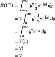
$$\begin{align*}E(Y^2) & = \int_{- \infty}^\infty y^2 \frac{1}{2} e^{- \lvert y ... ...y^2 e^{- y} \, d y \\ & = \Gamma(3) \\ & = 2 ! \\ & = 2 \end{align*}$$

(b)

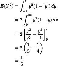
This density is symmetric about zero, hence the mean is zero and $\mathop{\rm var}\nolimits(Y) = E(Y^2)$. Now

$$\begin{align*}E(Y^2) & = \int_{- 1}^1 y^2 (1 - \lvert y \rvert) \, d y \\ &... ... = 2 \left(\frac{1}{3} - \frac{1}{4}\right) \\ & = \frac{1}{6} \end{align*}$$

(c)

This density is symmetric about 1/2, hence the mean is 1/2. Also

$$E(Y^2) = \int_0^1 y^2 6 y (1 - y) \, d y = 6 \int_0^1 y^3... ...ft[ \frac{y^4}{4} - \frac{y^5}{5} \right]_0^1 = \frac{6}{20}$$

Then

$$\mathop{\rm var}\nolimits(Y) = E(Y^2) - E(Y)^2 = \frac{6}{20} - \left(\frac{1}{2} \right)^2 = \frac{1}{20}$$

Problem L4-40ab

(a)

$$E(X) = 1 \times \frac{1}{2} + 3 \frac{1}{2} = 2$$

$$E(Y) = 0 \times \frac{1}{3} + 1 \times \frac{1}{3} + 2 \frac{1}{3} = 1$$

$$E(X^2) = 1^2 \times \frac{1}{2} + 3^2 \frac{1}{2} = 5$$

$$E(Y^2) = 0^2 \times \frac{1}{3} + 1^2 \times \frac{1}{3} + 2^2 \frac{1}{3} = \frac{5}{3}$$

$$\mathop{\rm var}\nolimits(X) = E(X^2) - E(X)^2 = 5 - 2^2 = 1$$

$$\mathop{\rm var}\nolimits(Y) = E(Y^2) - E(Y)^2 = \frac{5}{3} - 1^2 = \frac{2}{3}$$

$$E(XY) = (1 \times 2) \frac{1}{4} + (3 \times 1) \frac{1}{3} + (3 \times 2) \frac{1}{12} = 2$$

$$\mathop{\rm cov}\nolimits(X,Y) = E(XY) - E(X)E(Y) = 2 - 2 \times 1 = 0.$$

(the last result is obvious from symmetry).

(b)

$$\rho_{X,Y} = \frac{\mathop{\rm cov}\nolimits(X,Y)}{\sigma_X \sigma_Y} = 0$$

Problem N2-21

Since $X_1 + \cdots + X_n = 0$, we also have $\mathop{\rm var}\nolimits(X_1 + \cdots + X_n) = 0$, but

$$\mathop{\rm var}\nolimits(X_1 + \cdots + X_n) = n \mathop{\... ...\nolimits(X_1) + n (n - 1) \mathop{\rm cov}\nolimits(X_1, X_2)$$

by Theorem 2.22 in the notes. Hence

$$\mathop{\rm cov}\nolimits(X_1, X_2) = - \frac{1}{n - 1} \mathop{\rm var}\nolimits(X_1)$$

and

$$\mathop{\rm cor}\nolimits(X_1, X_2) = \frac{\mathop{\rm cov... ...1, X_2)}{\mathop{\rm var}\nolimits(X_1)} = - \frac{1}{n - 1}$$

Problem N2-22

Almost exactly the same calculation as the preceeding problem, except one starts with the inequality

$$\mathop{\rm var}\nolimits(X_1 + \cdots + X_n) \ge 0$$

and consequently derives an inequality.

Problem N2-24

This was CANCELLED, because it turned out to be messier than I thought.

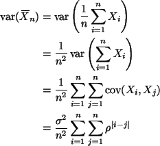
$$\begin{align*}\mathop{\rm var}\nolimits(X{\mkern -13.5 mu}\overline{\phantom{\te... ...igma^2}{n^2} \sum_{i=1}^n \sum_{j = 1}^n \rho^{\lvert i - j \rvert} \end{align*}$$
We can get rid of one sum. There are n terms with i = j hence $\rho^0$, and there are 2 (n - 1) terms with $i = j \pm 1$ hence $\rho^1$, and there are 2 (n - 2) terms with $i = j \pm 2$ hence $\rho^2$, and so forth to 2 terms with i = 1 and j = n or vice versa hence $\rho^{n - 1}$, thus
$$\begin{align*}\mathop{\rm var}\nolimits(X{\mkern -13.5 mu}\overline{\phantom{\te... ...}{n} \left(1 + 2 \sum_{k=1}^{n - 1} \frac{n - k}{n} \rho^k \right) \end{align*}$$
but this does not simplify any further, at least not using the geometric series.

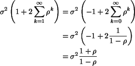
If anyone is wondering how I ever thought this was simple, I was recalling that the limit as n goes to infinity is simple

Using the linear combination form for variance, we have

$$\begin{align*}\lim_{n \to \infty} n \mathop{\rm var}\nolimits(X{\mkern -13.5 mu}... ...X}}}_n) & = \sigma^2 \left(1 + 2 \sum_{k=1}^\infty \rho^k \right) \end{align*}$$
because

$$\frac{n - k}{n} \to 1, \qquad \text{as $n \to \infty$}$$

and
$$\begin{align*}\sigma^2 \left(1 + 2 \sum_{k=1}^\infty \rho^k \right) & = \sigma... ...{1}{1 - \rho} \right) \\ & = \sigma^2 \frac{1 + \rho}{1 - \rho} \end{align*}$$
But we need to cover more material before we can get this far with this problem.

Problem N2-25

First we need to do the analogous equation for covariance, which isn't given in the notes or in Lindgren.
$$\begin{align*}cov(a + b X, c + d Y) & = E\{(a + b X - \mu_{a + b X}) (c + d Y ... ...\mu_X) (Y - \mu_Y)\} \\ & = b d \mathop{\rm cov}\nolimits(X, Y) \end{align*}$$
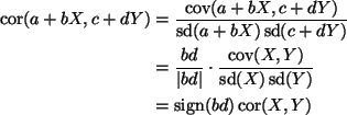
Then
$$\begin{align*}\mathop{\rm cor}\nolimits(a + b X, c + d Y) & = \frac{\mathop{\r... ... = \mathop{\rm sign}\nolimits(b d) \mathop{\rm cor}\nolimits(X, Y) \end{align*}$$

Problem N2-28

(a)

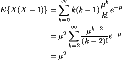
$$\begin{align*}E\{X (X - 1)\} & = \sum_{k = 0}^{\infty} k (k - 1) \frac{\mu^k}{... ... 2}^{\infty} \frac{\mu^{k - 2}}{(k - 2)!} e^{- \mu} \\ &= \mu^2 \end{align*}$$

(b)

We want to use

$$\mathop{\rm var}\nolimits(X) = E(X^2) - E(X)^2$$

and we can get E(X²) from part (a)

$$E\{X (X - 1)\} = E(X^2) - E(X) = \mu^2$$

so

$$E(X^2) = \mu^2 + \mu$$

and

$$\mathop{\rm var}\nolimits(X) = (\mu^2 + \mu) - \mu^2 = \mu$$

Problem N2-30

Note the density is

$$f(x) = \frac{1}{b - a}, \qquad a < x < b$$

because the length of the interval is b - a. This is symmetric about the midpoint of the interval (a + b) / 2, so that is the mean.

Then

$$E(X^2) = \frac{1}{b - a} \int_a^b x^2 \, d x = \frac{(b^3-a^3)}{3(b-a)} = \frac{b^2+ab+a^2}{3}$$

and
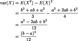
$$\begin{align*}\mathop{\rm var}\nolimits(X) & = E(X^2) - E(X)^2 \\ & = \fra... ...} \\ & = \frac{a^2-2ab+b^2}{12} \\ & = \frac{(b - a)^2}{12} \end{align*}$$

Problem N2-32

(a)

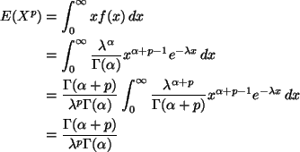
$$\begin{align*}E(X^p) & = \int_0^\infty x f(x) \, d x \\ & = \int_0^\infty ... ... d x \\ & = \frac{\Gamma(\alpha + p)}{\lambda^p \Gamma(\alpha)} \end{align*}$$
and this cannot be simplified if p is not an integer.

(b)

Using part (a) and the recursion formula for the gamma function, (B.2) in the appendix on ``brand name distributions'' of the notes, twice

$$E(X^2) = \frac{\Gamma(\alpha + 2)}{\lambda^2 \Gamma(\alpha)... ...da^2 \Gamma(\alpha)} = \frac{(\alpha + 1) \alpha}{\lambda^2}$$

and

$$\mathop{\rm var}\nolimits(X) = E(X^2) - E(X)^2 = \frac{(\alp... ...2} - \frac{\alpha^2}{\lambda^2} = \frac{\alpha}{\lambda^2}$$

Problem N2-33

(a)

The integral

$$\int_1^\infty x^{k} \frac{3}{x^4} \, d x = 3 \int_1^\infty x^{k - 4} \, d x$$

exists when k - 4 < - 1, that is, when k < 3. If $k \geq 3$, the integral does not exist (or is $+ \infty$).

The question asked about positive integers, so the answer is k = 1 or 2.

(b)

For k < 3

$$E(X^k) = 3 \int_1^\infty x^{k - 4} \, d x = \frac{3 x^{-4+k+1}}{-4+k+1} \biggr\vert _1^\infty = \frac{3}{3-k}$$

Note (not a part of the problem, but an interesting point) that the formula

$$E(X^k) = \frac{3}{3-k}$$

is completely bogus for k > 3. The formula gives a finite negative number for the expectation, which is ridiculous, the expectation of a positive random variable being positive. Of course, the expectation doesn't exist when k > 3, but (the point!) you can't tell that from looking at the formula for E(X^k) derived in this section. You have to do the thinking in part (a) not just plow ahead to part (b).

Problem N2-34

(a)

The integral

$$\int_0^1 x^k \frac{1}{2\sqrt{x}} \, d x = \frac{1}{2} \int_0^1 x^{k-1/2} \, d x$$

exists when k - 1 / 2 > - 1, which is true for all positive k.

Thus E(X^k) exists for k = 1, 2, $\ldots$ (all positive integers).

(b)

$$E(X^k) = \frac{1}{2} \int_0^1 x^{k-1/2} \, d x = \frac{... ...1/ 2} \biggr]_0^1 = \frac{1}{2(k+1/2)} = \frac{1}{2 k + 1}$$