Statistics 5101, Fall 2000, Geyer

Homework Solutions #3

Problem 3-12

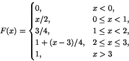
The completed definition of F

$$F(x) = \begin{cases} 0, & x < 0, \\ x/2, & 0 \leq x < 1, \... ... \\ 1+(x-3)/4, & 2 \leq x \leq 3,\\ 1, & x > 3 \end{cases}$$

(a)

P(X = 1/2)= 0, since if the c. d. f. is continuous a single value has probability zero.

(b)

P(X=1) = 1/4, the jump at x = 1/2.

(c)

P(X < 1) = F(1) - P(X=1) = 3/4 - 1/4 = 1/2.

(d)

F(X) = .25 at x = .5, so this is the first quartile.

F(X) = .75 for $x \in [1,2]$, so any number in [1,2] is a third quartile.

F(X) = .50 for x = 1, so that is the median.

(e)

$P( X \leq 1) = F(1) = 3/4$.

(f)

$P(X > 2) = 1 - P(X \leq 2) = 1 - F(2) = 1/4$.

(g)

$P(1/2 \leq X \leq 3/2) = F(3/2) - F(1/2) = 3/4 - 1/4 = 1/2$.

Problem 3-14

(a)

F(x) = .5, where $1 - \cos(x) = .5$, that is, $\cos(x) = .5$, and $x = \frac{\pi}{3}$.

Problem 3-19

(a)

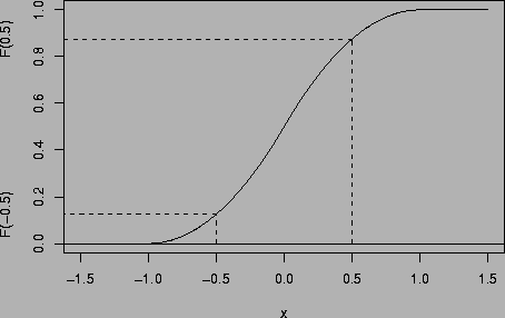
$P(\vert X\vert>1/2) = \frac{1/2 \times 1/2}{2} + \frac{1/2 \times 1/2}{2} = 1/4.$

 

Figure 1: The graph requested in 3-14 part (a).

(b)

For $x \leq -1$, the c. d. f. has value 0.

For -1 < x <0, the density function f(x)=1+x. Thus the c. d. f. F(x)can be obtained for any x between -1 and 0 by taking integral of the density function from 0 to an x between -1 and 0.

$$F(x) = \int_{\infty}^{x} (1+t) \, d t = \int_{-1}^{x} (1+... ... + \frac{x^{2}}{2} - (-1+\frac{1}{2}) = \frac{1}{2}(1+x)^{2}$$

Similarly, the c. d. f. F(x) for 0 < x < 1 is
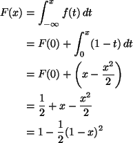
$$\begin{align*}F(x) & = \int_{-\infty}^{x} f(t) \, d t \\ & = F(0) + \int_{0... ...= \frac{1}{2} + x -\frac{x^2}{2} \\ & = 1-\frac{1}{2}(1-x)^{2} \end{align*}$$

 

Figure 2: The graph requested in 3-14 part (b). It is not clear how one is supposed to indicate the probability calculated in (a). It is F(- 0.5) + 1 - F(0.5), so we have indicated those two values of the distribution function.

Problem 3-23

As the hint says, assume without loss of generality that a = 0.
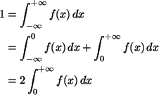
$$\begin{align*}1 & = \int_{-\infty}^{+ \infty} f(x) \, d x \\ & = \int_{-\i... ...t_0^{+ \infty} f(x) \, d x \\ & = 2 \int_0^{+\infty} f(x) \, d x \end{align*}$$
because f(x) = f(- x). From which we conclude

$$\int_0^{+\infty} f(x) \, d x = 1/2$$

as was to be proved.

Question:

What was that ``without loss of generality'' stuff in the hint? This is math jargon for saying that the proof of the special case a = 0 essentially proves the general case (because of something obvious, which is left unsaid, an exercise for the reader).

In this case, the something obvious is the change of variable theorem. If X is symmetric about a, then Y = X - a is symmetric about zero, and the special case that we just proved shows that Y has median zero. Then a change of variable back (X = Y + a) shows that X has median a.

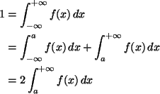
If you find that too confusing, you could just do the problem not using the hint, in which case the change of variables is explicit rather than implicit (hidden behind the ``without loss of generality'' woof). In general (not assuming a = 0)
$$\begin{align*}1 & = \int_{-\infty}^{+ \infty} f(x) \, d x \\ & = \int_{-\i... ...t_a^{+ \infty} f(x) \, d x \\ & = 2 \int_a^{+\infty} f(x) \, d x \end{align*}$$
because f(x + a) = f(a - x). Written out in detail

$$\int_a^{+\infty} f(x) \, d x = \int_0^{+\infty} f(a + t) \, d t$$

using the change of variable x = a + t, and
$$\begin{align*}\int_{-\infty}^a f(x) \, d x & = - \int_{+\infty}^0 f(a - t) \, d t \\ & = \int_0^{+\infty} f(a - t) \, d t \end{align*}$$
using the change of variable x = a - t.

Problem 3-24

Since f(x) should be a p. d. f., it must have the following properties.

1.

$f(x) \geq 0$, for all x, and

2.

$\int_{-\infty} ^{+ \infty} f(x)dx = 1$.

(a)

The first property checks if $k \ge 0$, because then $f(x) = kx \geq 0$.

The second property requires

$$1 = \int_{-\infty}^{+ \infty} f(x) \, d x = \int_0^2 k x \, d x = \frac{k x^2}{2} \bigg\vert _0^2 = 2 k$$

from which we conclude $k=\frac{1}{2}$.

(b)

The first property checks if $k \ge 0$, because then $f(x) = k x (1 - x) \geq 0$.

The second property requires

$$1 = \int_{-\infty} ^{+ \infty} f(x) \, d x = \int_0^1 k x... ...eft[ \frac{x^2}{2} - \frac{x^3}{3} \right]_0^1 = \frac{k}{6}$$

from which we conclude k = 6.

(c)

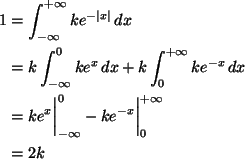
As with the other two parts any $k \ge 0$ satisfies the first property.

The second property requires
$$\begin{align*}1 & = \int_{-\infty}^{+\infty} k e^{-\lvert x \rvert} \, d x \\... ...ert _{-\infty}^0 - k e^{- x} \bigg\vert _0^{+\infty} \\ & = 2k \end{align*}$$
from which we conclude k = 1/2.

Problem 3-27

(a)

The marginal densities of U and V are

$$f_U(u) = \int_{0}^{\infty} f(u, v) \, d v = e^{-u}, \qquad u > 0.$$

and

$$f_V(v) = \int_{0}^{\infty} f(u, v) \, d u = e^{-v}, \qquad v > 0.$$

(b)

$$\mathop{\rm pr}\nolimits(U+V \leq 4) = \int_{0}^{4} \int_{0}^{4-v} e^{-(u+v)} \, d u \, d v = 1-5e^{-4}$$

(d)

$\mathop{\rm pr}\nolimits(U=V)=0$, because the integral over any set of area zero in two dimensions is zero, and the area of the line

$$\{\, (u, v) \in \mathbb{R} ^2 : u = v \,\}$$

is 0.

Problem 3-33

(a)

The transformation g defined by

$$g(x) = 2 \lvert x \rvert, \qquad \text{$- 1 < x < 0$ or $0 < x < 1$}$$

is noninvertible, but has two right inverses

$$h_-(y) = - \frac{y}{2}, \qquad 0 < y < 2$$

and

$$h_+(y) = \frac{y}{2}, \qquad 0 < y < 2$$

Thus Theorem 1.8 in the notes applies (this is much like Example 1.6.3 in the notes).

The derivatives are

$$\frac{d}{d y} h_{\pm}(y) = \pm \frac{1}{2}$$

and the $\mathcal{U}(-1, 1)$ distribution is symmetric, so if $Y = 2 \lvert X \rvert$
$$\begin{align*}f_Y(y) & = f_X(-y) \cdot \lvert - \tfrac{1}{2} \rvert + f_X(y) ... ...\rvert \\ & = f_X(y) \\ & = \tfrac{1}{2}, \qquad 0 < y < 2 \end{align*}$$
and we see $Y \sim \mathcal{U}(0, 2)$.

(b)

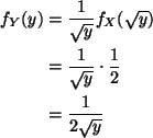
This part is even more like Example 1.6.3 in the notes. In fact, we can use Corollary 1.9.

If Y = X², then
$$\begin{align*}f_Y(y) & = \frac{1}{\sqrt{y}} f_X(\sqrt{y}) \\ & = \frac{1}{\sqrt{y}} \cdot \frac{1}{2} \\ & = \frac{1}{2 \sqrt{y}} \end{align*}$$
is the formula for the density. Of course, we aren't done until we attach the range of Y, which is clearly (0, 1). Thus

$$f_Y(y) = \frac{1}{2 \sqrt{y}}, \qquad 0 < y < 1$$

(c)

The transformation Y = (X + 1) / 2 is linear, so we can use Theorem 7 on p. 64 in Lindgren

$$f_Y(y) = f_X(2 y - 1) \cdot 2 = \frac{1}{2} \cdot 2 = 1$$

is the formula for the density. The range of Y is (0, 1). Hence $Y \sim \mathcal{U}(0,1)$.

Problem 3-37

The transformation

$$V = - \log X = g(X)$$

has inverse transformation

$$X = \exp(- V) = h(V)$$

which has derivative

h'(v) = - e^{- v}

So
$$\begin{align*}f_V(v) & = f_X[h(v)] \cdot \lvert h'(v) \rvert & = \theta (e^{... ...= \theta e^{- v (\theta - 1) - v} \\ & = \theta e^{- v \theta} \end{align*}$$
We also have to find the range of V. As x goes from zero to one, $\log(x)$ goes from $- \infty$ to zero, and $- \log(x)$ goes from $+ \infty$ to zero. Thus

$$f_V(v) = \theta e^{- v \theta}, \qquad 0 < v < \infty$$

Problem N1-1

Let Y=X³. The transformation g defined by g(x) = x³ is invertible with inverse h defined by

$$h(y) = y^{1 / 3}, \qquad y \in \mathbb{R}$$

and having derivative

$$h'(y) = \frac{1}{3} y^{- 2 / 3}.$$

Thus
$$\begin{align*}f_Y(y) & = f_X[h(y)] \cdot \lvert h'(y) \rvert \\ & = \frac{... ... \sqrt{2 \pi}} e^{- y^{2 / 3} / 2}, \qquad - \infty < y < + \infty \end{align*}$$

Problem N1-2

Let $Y=\sqrt{x}$. The transformation g defined by

$$g(x) = x^{1 / 2}, \qquad x > 0$$

is invertible with inverse h defined by

$$h(y) = y^2, \qquad y > 0$$

and having derivative

$$h'(y) = 2 y, \qquad y > 0.$$

Applying change of variable theorem, the density function of Y is

$$f_Y(y) = y^{5} e^{-y^2}, \qquad 0 < y < \infty.$$

Problem N1-3

The transformation
$$\begin{align*}U & = X + Y \\ V & = \frac{X}{X+Y} \end{align*}$$
has inverse transformation
$$\begin{align*}X & = U V \\ Y & = U (1 - V) \end{align*}$$
Note for future reference the ranges of the transformed variables
$$\begin{gather*}0 < U < \infty \\ 0 < V < 1 \end{gather*}$$
The derivative matrix is

$$\begin{pmatrix} \frac{\partial x}{\partial u} & \frac{\parti... ...\end{pmatrix} = \begin{pmatrix}v & u \\ 1-v & -u \end{pmatrix}$$

Thus the Jacobian is J(u,v) = -u v - u (1 - v) = - u, and the joint density function of U and V is

$$f_{U,V}(u,v) = \frac{1}{2} u^{2} e^{-u}, \qquad 0 < v < 1,\ 0 < u < \infty.$$

Note that this is a function of u and v despite having no v in the formula.