Stat 3011 Midterm 2 (Computer Part)

Problem 1

(a)

Rweb:> pt(-5, df=5) 
[1] 0.002052358

(b)

Rweb:> 1 - pt(1.5, df=5) 
[1] 0.09695184

(c)

Rweb:> 2 *(1 - pt(2.0, df=5)) 
[1] 0.1019395

(d)

Rweb:> -qt(0.05, df=5) 
[1] 2.015048

If $\mathop{\rm pr}\nolimits (\lvert T \rvert > t) = 0.10$, then there is probability 0.05 in the lower tail below $- t$, probability 0.05 in the upper tail above $+ t$, and probability 0.90 between $- t$ and $+ t$. Thus $- t$ is the 0.05 quantile and $+ t$ is the 0.95 quantile, and either

- qt(0.05, df=5)

or

qt(0.95, df=5)

gives the answer.

Problem 2

(a)

Rweb:> t.test(x, y, conf.level = 0.99) 
 
	Welch Two Sample t-test 
 
data:  x and y  
t = -0.1572, df = 4.569, p-value = 0.8818  
alternative hypothesis: true difference in means is not equal to 0  
99 percent confidence interval: 
 -0.04819463  0.04474463  
sample estimates: 
mean of x mean of y  
 1.097425  1.099150

The confidence interval $(-0.04819463, 0.04474463)$ calculated by R, should according to the rules in Section 7.4.3 in Wild and Seber be rounded to one more significant figure than the width of the interval. That's the fourth decimal place here, giving $(-0.0482, 0.0447)$ for the rounded interval.

(b)

Use of Studen't $t$ distribution always requires the assumption of normal population distributions.

Problem 3

(a)

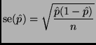
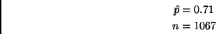
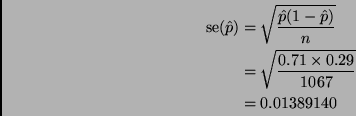
The formula for the standard error is

$$\mathop{\rm se}\nolimits (\hat{p}) = \sqrt{\frac{\hat{p} (1 - \hat{p})}{n}}$$

In this problem

$$\begin{split} \hat{p} & = 0.71 \\ n & = 1067 \end{split}$$

So

$$\begin{split} \mathop{\rm se}\nolimits (\hat{p}) & = \sqr... ...ac{0.71 \times 0.29}{1067}} \\ & = 0.01389140 \end{split}$$

So two standard errors is $2 \times 0.01389140 = 0.02778280$, and the two standard error interval is $0.71 \pm 0.028$ or $(0.682, 0.738)$.

An alternative solution that is not exactly what was asked, but is acceptable is

Rweb:> prop.test(1067 * 0.71, 1067) 
 
	1-sample proportions test with continuity correction 
 
data:  1067 * 0.71 out of 1067, null probability 0.5  
X-squared = 187.3797, df = 1, p-value = < 2.2e-16  
alternative hypothesis: true p is not equal to 0.5  
95 percent confidence interval: 
 0.6815786 0.7368888  
sample estimates: 
   p  
0.71

(b)

Everything is the same as in part (a) except now $\hat{p} = 0.91$ and $n = 67$. So

$$\begin{split} \mathop{\rm se}\nolimits (\hat{p}) & = \sqr... ...\frac{0.91 \times 0.09}{67}} \\ & = 0.03496267 \end{split}$$

So two standard errors is $2 \times 0.03496267 = 0.06992533$, and the two standard error interval is $0.91 \pm 0.070$ or $(0.840, 0.980)$.

An alternative solution that is not exactly what was asked, but is acceptable is

Rweb:> prop.test(67 * 0.91, 67) 
 
	1-sample proportions test with continuity correction 
 
data:  67 * 0.91 out of 67, null probability 0.5  
X-squared = 43.4257, df = 1, p-value = 4.404e-11  
alternative hypothesis: true p is not equal to 0.5  
95 percent confidence interval: 
 0.8082773 0.9627865  
sample estimates: 
   p  
0.91

(c)

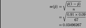
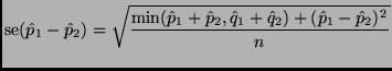
This is a ``type (c)'' problem in Wild and Seber's classification. The formula for the standard error is

$$\mathop{\rm se}\nolimits (\hat{p}_1 - \hat{p}_2) = \sqrt{\frac{\min(\hat{p}_1 + \hat{p}_2, \hat{q}_1 + \hat{q}_2) + (\hat{p}_1 - \hat{p}_2)^2}{n}}$$

where $\hat{q}_i = 1 - \hat{p}_i$. Rather than use the formula by hand, it is easier to use the box on the web page about this stuff.

Rweb:> p1 <- 0.77 
Rweb:> p2 <- 0.68 
Rweb:> n <- 1067 
Rweb:> (p1 - p2) + c(-1, 1) * 2 * 
+      sqrt((min(p1 + p2, 2 - p1 - p2) - (p1 - p2)^2) / n) 
[1] 0.04492794 0.13507206

Rounding to three significant figures we get $(0.045, 0.135)$. If you did do it by hand, the plus-or-minus form is $0.09 \pm 0.04507206$ or (rounded) $0.09 \pm 0.045$.

(Note: prop.test doesn't understand this kind of problem, so is useless here.)

(d)

Everything is the same as in part (c) except now $\hat{p}_1 = 0.95$, $\hat{p}_2 = 0.80$, and $n = 67$. So

Rweb:> p1 <- 0.95
Rweb:> p2 <- 0.80
Rweb:> n <- 67 
Rweb:> (p1 - p2) + c(-1, 1) * 2 * 
+      sqrt((min(p1 + p2, 2 - p1 - p2) - (p1 - p2)^2) / n) 
[1] 0.03345778 0.26654222

Rounding to three significant figures we get $(0.033, 0.267)$. If you did do it by hand, the plus-or-minus form is $0.09 \pm 0.1165422$ or (rounded) $0.09 \pm 0.117$.

(Note: prop.test doesn't understand this kind of problem, so is useless here.)