A confidence interval is an interval whose endpoints are statistics (numbers calculated from a random sample) whose purpose is to estimate a parameter (a number that could, in theory, be calculated from the population, if measurements were available for the whole population).
The confidence level of a confidence interval is the probability (conventionally expressed as a percent, though this is archaic) that the confidence interval actually contains the parameter.
A confidence interval has three elements. First there is the interval itself, something like (123, 456). Second is the confidence level, something like 95%. Third there is the parameter being estimated, something like the population mean μ. In order to have a meaningful statement, you need all three elements
(123, 456) is a 95% confidence interval for μ
(or something of the sort).
The three worst errors in statistics are (in order, starting with the worst).
The last mistake is the trickiest, and people who would never make mistakes 1 and 2 fall victim to 3. Here's a slogan that will help you remember.
It's called a 95% confidence interval because it misses 5% of the time.
A so-called margin of error
is not an absolute bound. A poll can
be wrong by more than that, and will be wrong by more than that 5% of the
time just by variability due to random sampling, and this is
even without taking biases into account (undercoverage,
nonresponse, response bias, wording of questions, see p. 185–189
in the textbook).
An improved slogan would be
It's called a 95% confidence interval because it misses 5% of the time, or more if there are any biases.
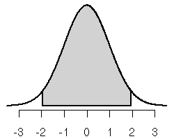
A standard backward lookup problem: find a number z* such that the probability that a normal random variable is less than z* standard deviations from its mean is 0.95.
Here's the picture for the standard normal distribution.
The gray shaded area is 0.95. By symmetry of the normal distribution, each unshaded tail area must be half of 1 − 0.95 = 0.05. Thus each is 0.05 ⁄ 2 = 0.025.
In order to look this up in a table we need to convert this into an
area to the left
problem. If we denote the left end of the shaded
gray area − z* and the right end z*, then
So we can backwards lookup 0.025 in the standard normal table to find − z* or backwards lookup 0.975 in the standard normal table to find z*. The relevant rows of the table are
         .00   .01   .02   .03   .04   .05   .06   .07   .08   .09
- 1.9 | .0287 .0281 .0274 .0268 .0262 .0256 .0250 .0244 .0239 .0233
  1.9 | .9713 .9719 .9726 .9732 .9738 .9744 .9750 .9756 .9761 .9767
Either lookup tells us that z* is 1.96.
This is a very important number called the z critical value (or normal critical value) for a 95% confidence interval.
We can also do this backwards lookup by computer as follows.
Table C in the insert with tables and formulas in our textbook (Moore) is mainly for so-called Student t critical values but also gives normal critical values in its bottom row.
z* | 0.674 0.841 1.036 1.282 1.645 1.960 2.054 2.326 2.576 2.807 3.091 3.291
      50%   60%   70%   80%   90%   95%   96%   98%   99%  99.5% 99.8% 99.9%
Here is a related question to that in the preceding section: find a number z* such that the probability that is less than z* of its standard deviations (σ ⁄ √n) from μ is 0.95.
If we assume the population is exactly normal, so the sampling distribution of is also exactly normal, then the answer is the same as in the preceding section z* = 1.96.
If the sample size is large then the answer from the preceding section will be a good approximation by the central limit theorem (regardless of whether the population distribution is normal or not).
If the sample size is large then it makes no difference whether we use σ ⁄ √n or s ⁄ √n (where σ is the population standard deviation and s is the sample standard deviation) by the law of large numbers.
If we assume the population is exactly normal and we know the population standard deviation, then
is an exact confidence interval for μ having the confidence level that goes with z*.
If the sample size is large then
is an approximate confidence interval for μ having the confidence level that goes with z*. The larger the sample size n, the better the approximation.
For this example, we use the data that is in the URL
so we can use the URL external data entry method.
If these data are a random sample from some population, then the result (40.57359, 54.15949) is a 95% confidence interval for the true unknown population mean μ.
There is no point in having so many significant figures. Usually we round the result, for example, to (40.6, 54.2) is a 95% confidence interval for μ.
How much you round depends on the purpose of the interval.
If instead we are given , s, and n, we do more or less the same thing. We just don't need a data URL.
Suppose we are told
and we want a 90% confidence interval for μ.
The sort of problem just above is easily done by hand calculation. We need to look up the appropriate normal critical value.
z* | 0.674 0.841 1.036 1.282 1.645 1.960 2.054 2.326 2.576 2.807 3.091 3.291
      50%   60%   70%   80%   90%   95%   96%   98%   99%  99.5% 99.8% 99.9%
Then the endpoints of the confidence interval are
(Just don't forget √n.)
When the sample size is not large, the error that results from using the sample standard deviation s where we should use the population standard deviation σ can be non-negligible.
In 1908 William Sealey Gosset published a solution to this problem.
If we assume the population is exactly normal, then the distribution of the sample mean standardized using the sample standard deviation
has a distribution that is not normal but was worked out by Gosset,
who wrote under the pseudonym Student
so the distribution is
called
the Student t distribution
for n − 1 degrees of freedom.
Calling a distribution after a letter is confusing, but there's nothing that can be done about it. It's not the stupidest name ever invented.
There is a different Student t distribution for each different sample size (each has a slightly different shape). The different Student t distributions are distinguished by a number called degrees of freedom, which in one-sample location problems is n − 1.
Naming these distributions by n − 1 rather than n is also confusing, but there's nothing that can be done about that either. This actually makes some sense, because the same distributions arise in inference for two samples (Chapter 17 in the textbook), for several samples (Chapter 22 in the textbook), and for least squares regression (Chapter 21 in the textbook), and the degrees of freedom is calculated differently in all these cases. We could have less confusion for one sample problems if we named these distributions for the one-sample sample size they are associated with, but that would cause more confusion later.
Student t distributions look more or less normal. They are
The plot made by the form below shows the standard normal density curve
(black) and the Student t distribution density curve (red)
for degrees of freedom determined by the df <- 5 statement
(which you can edit).
A computer simulation showing the t is actually correct (given its required assumptions) is on a web page for this class several years ago.
Everything in this section is very analogous to what we saw in the section on normal critical values. The only difference is that we use the t distribution instead of the z distribution (normal distribution).
Find the t critical value for a 95% confidence interval when there are only three data points, so there are n − 1 = 2 degrees of freedom.
The only things different are that we use the function qt
(on-line help)
rather than qnorm and there is an additional argument df that must be specified.
Table C in the textbook gives Student t critical values. Each row is for a different degrees of freedom (hence for a different distribution).
 2 | 0.816 1.061 1.386 1.886 2.920 4.303 4.849 6.965 9.925 14.09 22.33 31.60
      50%   60%   70%   80%   90%   95%   96%   98%   99%  99.5% 99.8% 99.9%
Everything in this section is very analogous to what we saw in the section on confidence intervals based on normal critical values. The only difference is that we use the t distribution instead of the z distribution (normal distribution).
If we assume the population is exactly normal then
is an exact confidence interval for μ having the confidence level that goes with the critical value t* for the Student t distribution with n − 1 degrees of freedom.
If the population distribution is close to normal, then the confidence interval above will be close to exact (a very good approximation), even for small sample sizes.
If the population distribution is far from normal, especially if very skewed, then the confidence interval above will be far from exact. Its actual confidence level will be far from its advertised confidence level.
The larger the sample size, the less the shape of the population distribution matters. Notice that the two confidence intervals
are the same except for critical values and that t critical values get closer and closer to z critical values as n goes to infinity (as we go down columns of Table C in the textbook). So there is hardly any difference between t and z confidence intervals for large n.
For this example, we use the data that is in the URL
so we can use the URL external data entry method.
These are the data for Example 13.3 where according to the story the
book tells the population standard deviation is known
, which is
almost never the case. Here we assume we know nothing about the population
other than our three measurements. Everything is the same as that example
except we use a t critical value instead of a z
critical value.
If these data are a random sample from an exactly normal population, then the result (0.8299960, 0.8508707) is a 95% confidence interval for the true unknown population mean μ.
There is no point in having so many significant figures. Usually we round the result, for example, to (0.830, 0.851) is a 95% confidence interval for μ.
How much you round depends on the purpose of the interval.
For this example, we use the data that is in the URL
so we can use the URL external data entry method. These are the data for Example 16.1 in the textbook.
If these data are a random sample from an exactly normal population, then the result (21.52709 29.80625) is a 95% confidence interval for the true unknown population mean μ.
This agrees with the interval calculated in the book except for rounding errors.
Here we redo the preceding example using an R function that does all the work of a t hypothesis test (which we haven't covered yet, Chapter 17 in the textbook) or confidence interval.
So long as we ignore all the output except the confidence interval, we will be O. K.
The only part of the output we currently know about is
95 percent confidence interval:
 21.52709 29.80625
which agrees with the calculation in the preceding section.
If instead we are given , s, and n, we do more or less the same thing. We just don't need a data URL.
Suppose we are told
and we want a 95% confidence interval for μ.
The sort of problem just above is easily done by hand calculation. We need to look up the appropriate Student t critical value (degrees of freedom is n − 1 = 17).
17 | 0.689 0.863 1.069 1.333 1.740 2.110 2.224 2.567 2.898 3.222 3.646 3.965
      50%   60%   70%   80%   90%   95%   96%   98%   99%  99.5% 99.8% 99.9%
Then the endpoints of the confidence interval are
In both cases, with computer or by hand, the same as we got when we analyzed the full data using the computer above.
The textbook has a section in Chapter 16 titled Robustness of t procedures, which is, when you think about it, fatuous. It says (p. 426)
Fortunately, the t procedures are quite robust against non-Normality of the population except when outliers or strong skewness are present.
Translation:
The t procedures never screw up except when they screw up.
Well, duh!
What is it about textbook authors that leads them to pontificate, oversimplifying to the point of silliness?
Gosset's invention, the Student
t distribution is
one of the really cool ideas of the 20th century. Saying silly things
about it doesn't make it any cooler.
When the population distribution is close to normal the t procedures work very well. When not, not. Heavy tails and heavy skewness are particularly devastating. Even one outlier can mess them up completely.
In this section we consider something completely different from all of
the statistical inference procedures in the textbook. The textbook
does have a companion chapter
on the CD-ROM, Chapter 23,
titled Nonparametric tests. But that chapter doesn't have
anything about confidence intervals, nor does it cover the simplest
nonparametric test, the so-called sign test, which is associated
with the confidence interval we present here.
Procedures like the one we present here that are very robust are traditionally
called nonparametric
even though they are about parameters. The
terminology doesn't really make sense, so don't worry about it.
When we first started talking about estimates of location (as statistical theory calls it) or of center (as elementary books call it) comparing the sample mean and the sample median, we learned that the sample mean is about as non-robust as an estimator can be — one outlier ruins it — whereas the sample median is about as robust as an estimator can be — a few outliers hardly affect it and even many outliers don't ruin it, so long as less than half the data are outliers.
Therefore, if we want robustness we had better avoid
and find something related to the median.
So that is what we now do. We will construct confidence intervals for the population median θ.
Suppose X1, …, Xn are a random sample from some continuous distribution.
We will assume continuous through this section (the rest of this web page). The point is that continuous random variables, if measured to enough decimal places, never come out exactly the same. Thus all of X1, …, Xn are different, and they are also different from the population mean θ (if measured to enough decimal places).
We make no other assumptions whatsoever about the population distribution.
Let
denote the data values in sorted order: X(1) is the smallest data value, X(2) is the next smallest, and so forth. (This is a standard convention. Parentheses around subscripts indicate sorted order.)
We consider confidence intervals constructed by counting the same number in from each end of the sequence of sorted data values, intervals of the form
By the complement rule and the addition rule
Now we need to recognize
And these are binomial probabilities: we have n IID trials and Xi is above or below θ with equal probability 1 ⁄ 2. Hence if Y is a binomial random variable with sample size n and success probability 1 ⁄ 2, then we have
Making no assumptions about the population distribution other than that it is continuous, (X(k + 1), X(n − k)) is a confidence interval for the population mean θ having confidence level
where Y is binomial with sample size n and success probability 1 ⁄ 2.
For this example, we redo the analysis done with a t procedure above, we use the data that is in the URL
First we choose a confidence level.
We can choose several confidence levels between 18.5% and 99.999%, but the only ones that are practically useful for most applications are 96.9% when k = 4 and 90.4% when k = 5.
Suppose we choose k = 4.
Conclusion: the interval (22, 33) is an exact 96.9% confidence interval for the population median θ. No assumptions about the shape of the population distribution are necessary.
In order to do a problem like this by hand, you need a table of the binomial distribution for the appropriate sample size and success probability, here n = 18 and for confidence intervals about the median the success probability is always 1 ⁄ 2.
Here is such a table (not complete — we need only the part for small k),
| k | 0 | 1 | 2 | 3 | 4 | 5 | 6 | 7 | 8 |
|---|---|---|---|---|---|---|---|---|---|
| P(Y ≤ k) | 0.0000 | 0.0001 | 0.0007 | 0.0038 | 0.0154 | 0.0481 | 0.1189 | 0.2403 | 0.4073 |
Now we need to calculate
for various values of k until we find a confidence level we like. As before, we decide on k = 4, which gives the confidence level 1 &minus 2 × 0.0154 = 0.9692, which is 96.92%.
For the next step we need the data in sorted order
11 12 14 18 22 22 23 23 26 27 28 29 30 33 34 35 35 40
We have highlighted the numbers k in from each end, which are the endpoints of the confidence interval.
The assumption that the population distribution is continuous means ties are impossible, but here we have ties. However, if we assume these data are rounded and before rounding were all different, we can see that if we had the unrounded data our confidence interval would be something like (22.23, 32.79) and what we now have is that unrounded interval rounded.
So our procedure is exact, even with ties, so long as we don't mind the inaccuracy introduced by rounding. And if we do mind, then why were the data rounded in the first place?
If the confidence interval presented in this section is so great (and it is),
why doesn't the textbook present it? In this respect, the textbook follows
the vast majority of intro stats textbooks. The sample mean gets the vast
majority of pages.
The sample median gets a brief mention in the descriptive
section in
the beginning. Nothing is said about inference for the median.
There are several justifications for this
efficient.
IMHO none of these reasons are any good. The justifications for presenting this interval are better.
In a nonparametric statistics course, like Stat 5601 here at the University of Minnesota, many other exact, robust procedures are covered, in particular, the procedures associated with the sign test presented above are covered in much more detail. A competing family of procedures, the procedures associated with the Wilcoxon signed rank test are also covered.