Stat 3011 Final Exam (Computer Part)

Problem 1

(a)

Rweb:> 1 - pnorm(67, 63.5, 2.5) 
[1] 0.08075666

(b)

Rweb:> pnorm(65, 63.5, 2.5) - pnorm(60, 63.5, 2.5) 
[1] 0.6449902

(c)

Rweb:> qnorm(0.80, 63.5, 2.5) 
[1] 65.60405

that is, 65.6 inches.

Problem 2

(a)

It is obvious that open is louder than closed or at least as loud. The only issue is whether there is enough data here to show that.

(b)

$$\begin{split} H_0 & : \mu_{\text{open}} = \mu_{\text{closed... ... H_1 & : \mu_{\text{open}} > \mu_{\text{closed}} \end{split}$$

where $\mu_{\text{open}}$ and $\mu_{\text{closed}}$ are the true population mean values of loudness under the two chewing conditions.

(c)

Rweb:> t.test(open, closed, alternative="greater") 
 
         Welch Two Sample t-test  
 
data:  open and closed  
t = 2.3194, df = 15.466, p-value = 0.01721  
alternative hypothesis: true difference in means is greater than 0  
95 percent confidence interval: 
 3.296907       NA  
sample estimates: 
mean of x mean of y  
    64.22     50.80

The $P$-value is $P = 0.01721$ (one-tailed).

If you did a two-tailed test, it would, of course, be double this.

(d)

This is a ``statistically significant'' difference in loudness using the conventional 0.05 criterion for significance. In fact, it is a good deal below this level, getting close to ``strong evidence'' in the terminology introduced by Wild and Seber on p. 379. What's between ``some'' and ``strong''? Perhaps ``fairly strong''?

However described in words, the $P$-value does indicate a difference in loudness between the chip chewing techniques.

Problem 3

(a)

This is a chi-square test for a two-way table. Because the row totals are fixed, this is a test of homogeneity of proportions rather than a test of independence.

(b)

The null hypothesis is that the probabilities in the two rows of the table are the same (box on p. 481 in Wild and Seber). The alternative is anything else (any difference between the probabilities in the two rows).

(c)

web:> chisq.test(data) 
 
         Pearson's Chi-square test  
 
data:  data  
X-squared = 84.4958, df = 4, p-value = < 2.2e-16

The $P$-value is $P \approx 10^{-16}$. (Of course, large sample approximation isn't that precise. All we really know is $P \approx 0$. Really small. But that's all we need to know.)

(d)

This says there is a highly statistically significant difference in opinions between consumers and dentists. The test doesn't say what the difference is, only that there is one. A glance at the table shows that consumers seem to like advertising more than dentists (at least did when the study was done 20 years ago), but the chi-square test doesn't say anything that precise.

Problem 4

(a)

(b)

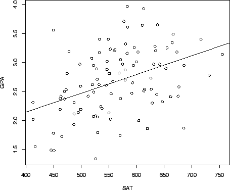
Rweb:> summary(out) 
 
Call: 
lm(formula = GPA ~ SAT) 
 
Residuals: 
     Min       1Q   Median       3Q      Max  
-1.21375 -0.35245  0.02555  0.35846  1.25487  
 
Coefficients: 
             Estimate Std. Error t value Pr(>|t|)     
(Intercept) 0.8474614  0.4058119   2.088   0.0394 *   
SAT         0.0032414  0.0007159   4.528 1.68e-05 *** 
--- 
Signif. codes:  0  `***'  0.001  `**'  0.01  `*'  0.05  `.'  0.1  ` '  1  
 
Residual standard error: 0.5269 on 98 degrees of freedom 
Multiple R-Squared: 0.173,      Adjusted R-squared: 0.1646  
F-statistic:  20.5 on 1 and 98 degrees of freedom,      p-value: 1.68e-05

The $P$-value for this test is the 1.68e-05 on the line labeled SAT, which means $P = 1.68 \times 10^{-5}$. The same $P$-value applies to

• test of no linear relationship
• test of zero slope
• test of zero correlation

All three are the same test with the same test statistic and the same $P$-value.

Since $P$ is very small, this is a highly statistically significant linear relationship.

(c)

Rweb:> predict(out, data.frame(SAT=650), interval="prediction") 
          fit      lwr      upr 
[1,] 2.954386 1.896076 4.012697

The interval is $(1.896076, 4.012697)$ or nicely rounded, $(1.90, 4.01)$.