Stat 5102 (Geyer) Final Exam
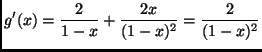
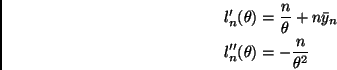
Looking at the simplest moment first,

The formula for ![]() should be familiar. It defines the location-scale
family with base density
should be familiar. It defines the location-scale
family with base density ![]() (Sections 4.1 and 9.2 of the course notes).
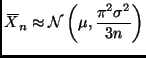
The variables
(Sections 4.1 and 9.2 of the course notes).
The variables

![]() is asymptotically normal with variance
is asymptotically normal with variance


Things are only a little different if we don't realize we can give the
answer for
![]() and
and
![]() instead of
instead of
![]() and
and
![]() .
.
Since
![]() ,
,
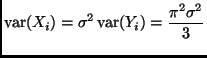
Note that ![]() is symmetric about zero but
is symmetric about zero but ![]() is symmetric about
is symmetric about ![]() ,
so
,
so ![]() is both the population mean and the population median. And
the asymptotic variance of
is both the population mean and the population median. And
the asymptotic variance of
![]() is
is
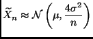
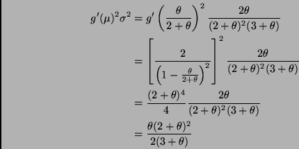
We need to apply the delta method to the estimator
![]() , where
, where

Because
![]() is a method of moments estimator it must have
asymptotic mean
is a method of moments estimator it must have
asymptotic mean ![]() (you can check this if you like, but it is
already part of the question statement and thus not a required calculation
in the answer).
(you can check this if you like, but it is
already part of the question statement and thus not a required calculation
in the answer).
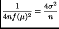
The asymptotic variance is
If anyone is wondering whether sample size one is ``large,'' recall that a single Poisson random variable is approximately normal if the mean is large (Section F.3 in the appendices of the notes).
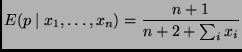
The obvious point estimate of
![]() is
is
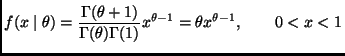
The density of the data is
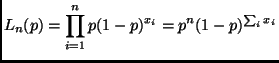
The likelihood for a sample of size ![]() is
is
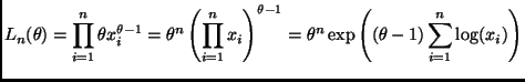
The log likelihood is thus
The likelihood is
The models in question have polynomials of degree 1, 2, 3, 4, and 5 as regression functions.
To be more precise, the regression functions are of the form
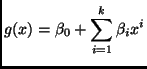
Because linear functions are special cases of quadratic, and so forth.
You obtain the models of lower degree by setting the coefficients of
higher powers of ![]() to zero in the larger models.
to zero in the larger models.
Starting at the bottom of the ANOVA table and reading up
Thus we conclude that the cubic model (Model 3) is correct, which means its
supermodels (Model 4 and Model 5) must also be correct. Or to be more finicky
we conclude that these data do not give any evidence that these models are
incorrect. And we conclude that the quadratic model (Model 2) and its submodel
(Model 1) are incorrect. The evidence for that latter conclusion is very
strong (repeating what was said above,
![]() ).
).
Many people were confused by ``correct'' and ``incorrect.'' If a model is correct, then so is every supermodel. If a model is incorrect, then so is every submodel. Hence in a nested sequence of models, there is a smallest correct model (here model 3) and all the models above it are also correct, but all the models below it are incorrect.
![\begin{displaymath}
\begin{split}
f(y \mid p)
& =
p (1 - p)^{y - 1}
\\
& ...
...1 - p)]
\\
& =
\exp[y \log(1 - p) + \logit(p)]
\end{split}\end{displaymath}](img56.png)
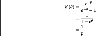
This clearly fits the form of equation (12.78) in the notes with
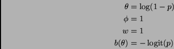
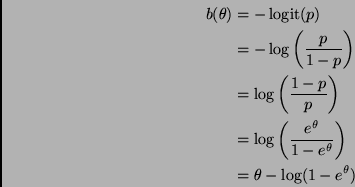
Of course, the last equation doesn't by itself define ![]() . To
do that we need to know
. To
do that we need to know ![]() as a function of
as a function of ![]() , that is, we have
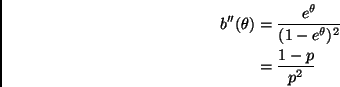
to solve the first equation above for
, that is, we have
to solve the first equation above for ![]() giving
giving
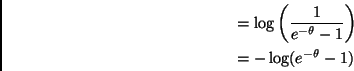
This is just added for my curiosity and perhaps to go in the homework problems some future semester.