Stat 5102 (Geyer) Midterm 1

Problem 1

(a)

The joint density is

$$f(\mathbf{x} \mid \theta) = \prod_{i = 1}^n \theta x_i^{\theta - ... ...ta^n \left(\prod_{i = 1}^n x_i\right)^{\theta - 1} = \theta^n a_n^{\theta - 1}$$

where for convenience we have defined

$$a_n = \prod_{i = 1}^n x_i$$

That is also the likelihood when considered a function of $\theta$ rather than $\mathbf{x}$. The prior density is

$$g(\theta) = \lambda e^{- \lambda \theta}$$

Hence the unnormalized posterior is likelihood$\times$   prior

$$h(\theta \mid \mathbf{x}) \propto \theta^n a_n^{\theta - 1} \cdot... ...\theta} = \frac{\lambda}{a_n} \theta^n e^{- \lambda \theta + \theta \log(a_n)}$$

This is clearly an unnormalized Gam$(n + 1, \lambda - \log a_n)$ density. So that is the posterior distribution.

(b)

Equation (11.36) in the notes gives the mode of the gamma distribution: shape parameter minus one over scale parameter, in this case

$$\frac{n}{\lambda - \log a_n}$$

Problem 2

(a)

By Example 11.2.4 in the notes, the posterior distribution is Normal$(a, b^{-1})$ where

$$\begin{split} a & = \frac{n \lambda \bar{x}_n + \lambda_0 \... ...mbda + \lambda_0} \\ b & = n \lambda + \lambda_0 \end{split}$$

and where $\lambda$, $\mu_0$, and $\lambda_0$ are the precision of the data distribution and the mean and precision of the prior distribution, respectively. Since the variances are $4$ and $1$, the precisions are $\lambda = 1 / 4$ and $\lambda_0 = 1$. Also $\mu_0 = 0$. Plugging those in gives

$$\begin{split} a & = \frac{n \bar{x}_n}{n + 4} \\ b & = \frac{n + 4}{4} \end{split}$$

(b)

The HPD region for a normal posterior distribution is

   posterior mean$$\pm 1.96 \times$$   posterior standard deviation$$$$

which in this case is

$$\frac{n \bar{x}_n}{n + 4} \pm 1.96 \sqrt{\frac{4}{n + 4}}$$

(recall that $b$ is posterior precision, which is one over posterior variance).

Problem 3

(a)

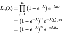
The likelihood for $\lambda$ is

$$\begin{split} L_n(\lambda) & = \prod_{i=1}^n \left(1 - e^... ... - e^{- \lambda}\right)^n e^{- n \lambda \bar{x}_n} \end{split}$$

The log likelihood is

$$\begin{split} l_n(\lambda) & = - n \lambda \bar{x}_n + n \log\left(1 - e^{- \lambda}\right) \end{split}$$

and

$$l_n'(\lambda) = - n \bar{x}_n + n \frac{e^{- \lambda}}{1 - e^{- \lambda}}$$

which is equal to zero when

$$\bar{x}_n = \frac{e^{- \lambda}}{1 - e^{- \lambda}} = \frac{1}{e^{\lambda} - 1}$$

Solving for $\lambda$ gives

$$\hat{\lambda}_n = \log\left(1 + \frac{1}{\bar{x}_n}\right)$$

(b)

$$\begin{split} l_1''(\lambda) & = - \frac{e^{- \lambda} (1... ... & = - \frac{e^{- \lambda}}{(1 - e^{- \lambda})^2} \end{split}$$

Since this does not contain $X_i$, it is nonrandom, and hence its negative is the Fisher information

$$I_1(\lambda) = \frac{e^{- \lambda}}{(1 - e^{- \lambda})^2}$$

and the Fisher information for a sample of size $n$ is $I_n(\lambda) = n I_1(\lambda)$.

(c)

A 95% C. I. for $\theta$ is

$$\hat{\lambda}_n \pm 1.96 \frac{1}{\sqrt{I_n(\hat{\lambda}_n)}}$$

Problem 4

Equation (10.37) in the notes gives the log likelihood for the two-parameter normal. To convert to the log likelihood for this problem we need to plug in $\theta$ for both $\mu$ and $\sigma$ giving

$$l_n(\theta) = - n \log(\theta) - \frac{1}{2 \theta^2} \sum_{i = 1}^n (x_i - \theta)^2$$ (1)

and derivatives

$$\begin{split} l_n'(\theta) & = - \frac{n}{\theta} + \fra... ... \frac{3}{\theta^4} \sum_{i = 1}^n (x_i - \theta)^2 \end{split}$$

The observed Fisher information is

$$J_n(\theta) = - l_n''(\theta) = \frac{4}{\theta^3} \sum_{i = 1}^n (x_i - \theta) + \frac{3}{\theta^4} \sum_{i = 1}^n (x_i - \theta)^2$$

Because $E(X_i - \theta) = 0$ and $E\{(X_i - \theta)^2\} = \theta^2$, the expected Fisher information is

$$I_n(\theta) = E\{J_n(\theta)\} = \frac{3 n}{\theta^2}$$

Alternate Solution

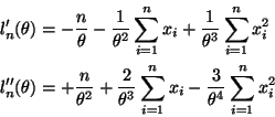
The solution given above is perhaps the easiest. Another contender for the easiest expands the binomial in (1) giving

$$l_n(\theta) = - n \log(\theta) - \frac{n}{2} + \frac{1}{\theta} \sum_{i = 1}^n x_i - \frac{1}{2 \theta^2} \sum_{i = 1}^n x_i^2$$

and derivatives

$$\begin{split} l_n'(\theta) & = - \frac{n}{\theta} - \fra... ...1}^n x_i - \frac{3}{\theta^4} \sum_{i = 1}^n x_i^2 \end{split}$$

So the observed Fisher information is

$$J_n(\theta) = - l_n''(\theta) = - \frac{n}{\theta^2} - \frac{2}{\theta^3} \sum_{i = 1}^n x_i + \frac{3}{\theta^4} \sum_{i = 1}^n x_i^2$$

Because $E(X_i) = \theta$ and $E(X_i^2) = \var(X_i) + E(X_i)^2 = 2 \theta^2$, the expected Fisher information is

$$I_n(\theta) = E\{J_n(\theta)\} = \frac{3 n}{\theta^2}$$

The deriviatives are a bit easier and the expectations are a bit harder than the first solution, but both are fairly easy.

More Alternate Solutions

The alternate solution that uses the empirical parallel axis theorm to ``simplify'' (1) giving

$$l_n(\theta) = - n \log(\theta) - \frac{n}{2 \theta^2} \sum_{i = 1}^n [ v_n + (\bar{x}_n - \theta)^2 ]$$ (2)

actually anti-simplification, because this doesn't simplify any derivatives and makes the expectations a lot harder.

$$\begin{split} E(V_n) & = \frac{n - 1}{n} \theta \\ E\{(X... ...\overline{\phantom{\text{X}}}_n) = \frac{\theta}{n} \end{split}$$

The alternate solution that expands the binomial in (2) giving

$$l_n(\theta) = - n \log(\theta) - \frac{n}{2} + \frac{n \bar{x}_n}{\theta} - \frac{n (v_n + \bar{x}_n^2)}{2 \theta^2}$$

further complicates the expectations although the derivatives are somewhat simplified. Now in addition to $E(V_n)$ given above we need

$$\begin{split} E(X{\mkern -13.5 mu}\overline{\phantom{\text{... ...t{X}}}_n)^2 \\ & = \frac{\theta^2}{n} + \theta^2 \end{split}$$

We won't give all the details. Of course $I_n(\theta)$ must be the same no matter how calculated (as long as no mistakes are made). For observed Fisher information we get

$$\begin{split} J_n(\theta) & = \frac{4 n}{\theta^3} (\bar{... ...eta^3} + \frac{3 n (v_n + \bar{x}_n)^2 }{\theta^4} \end{split}$$

Problem 5

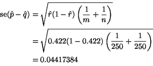
Example 9.5.4 in the notes gives the math for this problem. The natural estimates of $p$ and $q$ are $\hat{p} = 0.38$ and $\hat{q} = 0.464$. The natural test statistic is $\hat{p} - \hat{q}$ divided by its standard error (estimated standard deviation). As explained in the example, the natural choice for the standard error when we assume $p = q$ uses the pooled estimate of $p$ (and $q$), which is

$$\hat{r} = \frac{m \hat{p} + n \hat{q}}{m + n} = \frac{250 \cdot 0.38 + 250 \cdot 0.464}{250 + 250} = \frac{0.38 + 0.464}{2} = 0.422$$

Then the standard error is

$$\begin{split} \se(\hat{p} - \hat{q}) & = \sqrt{\hat{r} (1... ...250} + \frac{1}{250}\right)} \\ & = 0.04417384 \end{split}$$

So the test statistic is

$$z = \frac{\hat{p} - \hat{q}}{\se(\hat{p} - \hat{q})} = \frac{0.38 - 0.464}{0.04417384} = -1.9016$$

which has an asymptotic standard normal distribution under $H_0$. The $P$-value for this (one-tailed, lower tailed) test is the area under the standard normal curve to the left of $z$, which is

$$\Phi(z) = .0287$$

(no interpolation necessary since $z$ is so close to 1.900).

Not part of the question, but of interest in real life is the interpretation of the $P$-value. According to conventional standards of evidence, this is a ``statistically significant'' result because $P < .05$. Since $P = .029$ is not that far below .05, this is not absolutely compelling evidence of effectiveness of the new treatment, but it is fairly compelling.

Alternate Calculation of $\hat{r}$

The pooled estimator of $p$ and $q$ under $H_0$ is just the number of deaths in both groups divided by the number of subjects in both groups, so is also

$$\hat{r} = \frac{95 + 116}{250 + 250} = 0.422$$

Alternate Solution

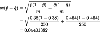
An asymptotically equivalent way to do the problem (almost no difference when $m$ and $n$ are large and $H_0$ is true) uses the standard error estimate

$$\begin{split} \se(\hat{p} - \hat{q}) & = \sqrt{\frac{\hat... ...rac{0.464 (1 - 0.464)}{250}} \\ & = 0.04401382 \end{split}$$

So the test statistic is

$$z = \frac{\hat{p} - \hat{q}}{\se(\hat{p} - \hat{q})} = \frac{0.38 - 0.464}{0.04401382} = -1.9085$$

giving a $P$-value

$$\Phi(z) = .0282$$

(or .0281 if you don't interpolate).

Note that this method is not recommended in real life, not because there is anything wrong with it, but because it's not the method taught in intro statistics books and hence people will argue.