next_group up previous
Up: Stat 5102

Stat 5102 (Geyer) Midterm 1

Problem 1

The basic fact this problem uses is

$\displaystyle \frac{X{\mkern -13.5 mu}\overline{\phantom{\text{X}}}_n - \mu}{S_n / \sqrt{n}} \sim t(n - 1)
$

(Corollary 7.25 in the notes), which, since $ \mu = 0$, specializes to

$\displaystyle \frac{X{\mkern -13.5 mu}\overline{\phantom{\text{X}}}_n}{S_n / \sqrt{n}} \sim t(n - 1)$ (1)

in this problem. This is the only exact result we have involving both $ X{\mkern -13.5 mu}\overline{\phantom{\text{X}}}_n$ and $ S_n$, so nothing else is of any use.

To use (1), we must put the event of interest $ X{\mkern -13.5 mu}\overline{\phantom{\text{X}}}_n < S_n$ in a form related to the left hand side of (1). Clearly, this is equivalent to

$\displaystyle \frac{X{\mkern -13.5 mu}\overline{\phantom{\text{X}}}_n}{S_n / \sqrt{n}}
<
\sqrt{n}
=
3
$

So the probability we need to find $ P(Y < 3)$ where $ Y$ is a $ t(n - 1)$ random variable ($ n - 1 = 8$ degrees of freedom).

From Table IIIa in Lindgren $ P(Y > 3) = 0.009$, so $ P(Y < 3) = 1 - 0.009 = 0.991$.

Problem 2

To use the method of moments, we first need to find some moments. Since this is not a ``brand name'' distribution, we must integrate to find the moments. The obvious moment to try first is the first moment (the mean)

\begin{displaymath}
\begin{split}
\mu
& =
\int_0^1 x f_\beta(x) \, d x
\\
...
...ht]_0^1
\\
& =
\frac{1 + 2 \beta}{3 + 3 \beta}
\end{split}\end{displaymath}

Solving for $ \beta$ as a function of $ \mu$, we get

$\displaystyle \beta = \frac{3 \mu - 1}{2 - 3 \mu}
$

(the numerator and denominator are both positive because $ 1 / 3 < \mu < 2 / 3$.)

Either way, we get a method of moments estimator by plugging in $ X{\mkern -13.5 mu}\overline{\phantom{\text{X}}}_n$ for $ \mu$

$\displaystyle \hat{\beta}_n = \frac{3 X{\mkern -13.5 mu}\overline{\phantom{\text{X}}}_n - 1}{2 - 3 X{\mkern -13.5 mu}\overline{\phantom{\text{X}}}_n}
$

Problem 3

(a)

The asymptotic distribution of $ X{\mkern -13.5 mu}\overline{\phantom{\text{X}}}_n$ is, as usual, by the CLT,

$\displaystyle X{\mkern -13.5 mu}\overline{\phantom{\text{X}}}_n \approx \NormalDis\left(\mu, \frac{\sigma^2}{n}\right).
$

Plugging in $ \sigma^2 = \mu$ gives

$\displaystyle X{\mkern -13.5 mu}\overline{\phantom{\text{X}}}_n \approx \NormalDis\left(\mu, \frac{\mu}{n}\right).
$

(b)

The asymptotic distribution of $ V_n$ is, by Corollary 7.17 in the notes,

$\displaystyle V_n
\approx
\NormalDis\biggl(\mu_2, \frac{\mu_4 - \mu_2^2}{n}\biggr).
$

where $ \mu_2 = \sigma^2 = \mu$ and $ \mu_4 = \mu + 3 \mu^2$ are given in the problem statement. Plugging these in gives

$\displaystyle V_n
\approx
\NormalDis\biggl(\mu, \frac{\mu + 2 \mu^2}{n}\biggr).
$

(c)

The ARE is the ratio of the asymptotic variances, either $ 1 + 2 \mu$ or the the reciprocal $ 1 / (1 + 2 \mu)$, depending on which way you write it.

(d)

The better estimator is the one with the smaller asymptotic variance, in this case $ X{\mkern -13.5 mu}\overline{\phantom{\text{X}}}_n$.

Problem 4

This is a problem for the delta method. We know from the properties of the exponential distribution

$\displaystyle E(X_i) = \frac{1}{\lambda}
$

and

$\displaystyle \var(X_i) = \frac{1}{\lambda^2}
$

Hence the CLT says in this case

$\displaystyle X{\mkern -13.5 mu}\overline{\phantom{\text{X}}}_n
\approx
\NormalDis\left(\frac{1}{\lambda}, \frac{1}{n \lambda^2}\right)
$

For any differentiable function $ g$, the delta method says

$\displaystyle g(X{\mkern -13.5 mu}\overline{\phantom{\text{X}}}_n)
\approx
\Nor...
...\lambda}\Bigr),
g'\Bigl(\frac{1}{\lambda}\Bigr)^2 \frac{1}{n \lambda^2}\right)
$

The $ g$ such that $ W_n = g(X{\mkern -13.5 mu}\overline{\phantom{\text{X}}}_n)$ is

$\displaystyle g(x) = \frac{x}{1 + x}$ (2)

which has derivative

$\displaystyle g'(x) = \frac{1}{(1 + x)^2}$ (3)

so

$\displaystyle g\Bigl(\frac{1}{\lambda}\Bigr) = \frac{1}{1 + \lambda}
$

and

$\displaystyle g'\Bigl(\frac{1}{\lambda}\Bigr) = \frac{\lambda^2}{(1 + \lambda)^2}
$

and

$\displaystyle W_n
\approx
\NormalDis\left(\frac{1}{1 + \lambda},
\frac{\lambda^2}{n (1 + \lambda)^4} \right)
$

Problem 5

There are several different ways to proceed here.

Using a Confidence Interval for the Mean

The mean is $ \mu = 1 / p$. Thus we could just get a confidence interval for $ \mu$ and take reciprocals of the endpoints to get a confidence interval for $ p$.

A confidence interval for $ \mu$ can be found using Theorem 9.8 in the notes. From Section B.1.8 of the notes

$\displaystyle \var(X_i) = \frac{1 - p}{p^2} = \mu (\mu - 1)
$

so by the LLN and the continuous mapping theorem

$\displaystyle S_n = \sqrt{X{\mkern -13.5 mu}\overline{\phantom{\text{X}}}_n (X{\mkern -13.5 mu}\overline{\phantom{\text{X}}}_n - 1)}
$

is a consistent estimator of the population standard deviation $ \sigma$ needed for the theorem. The theorem gives

$\displaystyle X{\mkern -13.5 mu}\overline{\phantom{\text{X}}}_n \pm 1.96 \sqrt{...
...ntom{\text{X}}}_n (X{\mkern -13.5 mu}\overline{\phantom{\text{X}}}_n - 1)}{n}}
$

as an asymptotic 95% confidence interval for $ \mu$. So

$\displaystyle \frac{1}{X{\mkern -13.5 mu}\overline{\phantom{\text{X}}}_n + 1.96...
...tom{\text{X}}}_n (X{\mkern -13.5 mu}\overline{\phantom{\text{X}}}_n - 1)}{n}}}
$

is an asymptotic 95% confidence interval for $ p = 1 / \mu$. Plugging in the numbers gives

$\displaystyle 0.180 < p < 0.256
$

Using the Delta Method

The obvious point estimator for $ p$ is

$\displaystyle \hat{p}_n = \frac{1}{X{\mkern -13.5 mu}\overline{\phantom{\text{X}}}_n}
$

The CLT says

$\displaystyle X{\mkern -13.5 mu}\overline{\phantom{\text{X}}}_n \approx \NormalDis\left( \frac{1}{p}, \frac{(1 - p)}{n p^2} \right)
$

Applying the delta method with the transformation

$\displaystyle g(u) = \frac{1}{u}
$

with derivative

$\displaystyle g'(u) = - \frac{1}{u^2}
$

gives

$\displaystyle g\Bigl(\frac{1}{p}\Bigr) = p
$

and

$\displaystyle g'\Bigl(\frac{1}{p}\Bigr) = - p^2
$

and

$\displaystyle \hat{p}_n \approx \NormalDis\left( p, \frac{p^2 (1 - p)}{n} \right)
$

which gives an asymptotic 95% confidence interval

$\displaystyle \hat{p}_n \pm 1.96 \sqrt{\frac{\hat{p}_n^2 (1 - \hat{p}_n)}{n}}
$

Plugging in the numbers gives

$\displaystyle 0.2114 \pm 0.03680
$

or

$\displaystyle 0.1746 < p < 0.2482
$

which is pretty close to the other interval.

Solving Quadratic Inequalities

The really hard way to do this problem is to start with

$\displaystyle X{\mkern -13.5 mu}\overline{\phantom{\text{X}}}_n \approx \NormalDis\left(\frac{1}{p}, \frac{1 - p}{n p^2}\right)
$

and standardize giving the asymptotically standard normal quantity

$\displaystyle \frac{X{\mkern -13.5 mu}\overline{\phantom{\text{X}}}_n - \frac{1}{p}}{\sqrt{\frac{1 - p}{n p^2}}}
$

from which we conclude that the set of $ p$ such that

$\displaystyle \left\lvert \frac{X{\mkern -13.5 mu}\overline{\phantom{\text{X}}}_n - \frac{1}{p}}{\sqrt{\frac{1 - p}{n p^2}}}
\right\rvert < 1.96
$

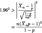
is an asymptotic 95% confidence interval for $ p$. It turns out this is solvable, equivalent to

\begin{displaymath}
\begin{split}
1.96^2 & >
\left\lvert \frac{X{\mkern -13.5 ...
...mu}\overline{\phantom{\text{X}}}_n p - 1)^2}{1 - p}
\end{split}\end{displaymath}

Or, writing $ z = 1.96$, we see the confidence interval has endpoints satisfying the quadratic equation

$\displaystyle (1 - p) z^2 = n (X{\mkern -13.5 mu}\overline{\phantom{\text{X}}}_n p - 1)^2
$

which has roots

$\displaystyle \frac{2 n X{\mkern -13.5 mu}\overline{\phantom{\text{X}}}_n - z^2...
...antom{\text{X}}}_n}}
{2 n X{\mkern -13.5 mu}\overline{\phantom{\text{X}}}_n^2}
$

or

$\displaystyle 0.17375 < p < 0.247366
$


next_group up previous
Up: Stat 5102
Charles Geyer
2001-03-05