Stat 5102 (Geyer) Final Exam

Problem 1

First define
$$\begin{align*}\mu & = \frac{\alpha}{\lambda} \\ \sigma^2 & = \frac{\alpha}{\lambda^2} \end{align*}$$
so
$$\begin{align*}E(X_i) & = \mu \\ \var(X_i) & = \sigma^2 \end{align*}$$
and the CLT says

$$\sqrt{n} \left(X{\mkern -13.5 mu}\overline{\phantom{\text{X}}... ...hcal{D}}{\longrightarrow} \NormalDis\left(0, \sigma^2\right).$$

Now we apply the delta method to the transformation

$$g(x) = \log(x)$$

because the random variable we want the the asymptotic of is $g(X{\mkern -13.5 mu}\overline{\phantom{\text{X}}}_n)$. This has derivative

$$g'(x) = \frac{1}{x}$$

Hence the delta method says

$$\sqrt{n} \left[ g(X{\mkern -13.5 mu}\overline{\phantom{\text{... ...longrightarrow} \NormalDis\left(0, g'(\mu)^2 \sigma^2 \right)$$

Now

$$g'(\mu)^2 \sigma^2 = \left(\frac{\lambda}{\alpha}\right)^2 \frac{\alpha}{\lambda^2} = \frac{1}{\alpha}$$

and

$$g(\mu) = \log(\alpha) - \log(\lambda)$$

Hence

$$\sqrt{n} \left[ \log(X{\mkern -13.5 mu}\overline{\phantom{\te... ...ckrel{\mathcal{D}}{\longrightarrow} \NormalDis(0, 1 / \alpha)$$

or

$$\log(X{\mkern -13.5 mu}\overline{\phantom{\text{X}}}_n) \appr... ...left(\frac{\alpha}{\lambda}\right), \frac{1}{n \alpha} \right)$$

Problem 2

Let's look at the simplest moment first

$$E(X_i) = \frac{s}{s + t} = \theta$$

Thus

$$\hat{\theta}_n = X{\mkern -13.5 mu}\overline{\phantom{\text{X}}}_n$$

is a perfectly good method of moments estimator of $\theta$. The CLT gives its asymptotic distribution

$$\hat{\theta}_n \approx \NormalDis(\theta, \sigma^2 / n)$$

where

$$\sigma^2 = \var(X_i) = \frac{s t}{(s + t + 1) (s + t)^2} = \frac{\theta (1 - \theta)}{2}$$

Problem 3

An asymptotic test can be based on the asymptotically pivotal quantity

$$Z = \frac{X{\mkern -13.5 mu}\overline{\phantom{\text{X}}}_n - \mu}{S_n / \sqrt{n}}$$

which is approximately standard normal for large n, where S_nis the sample standard deviation (the ``plug-in'' theorem allows any consistent estimator of the population standard deviation $\sigma$, but the convenient one here is S_n). To do the test in this particular problem we need the mean of the beta distribution (from p. 176 in Lindgren)

$$\mu = \frac{s}{s + t} \\$$

So under H₀ (s = t)

$$\mu = \frac{1}{2} \\$$

That's the value of $\mu$ that we plug in to compute Z

$$Z = \frac{X{\mkern -13.5 mu}\overline{\phantom{\text{X}}}_n -... ...n / \sqrt{n}} = \frac{0.57 - 0.50}{\sqrt{0.036 / 100}} = 3.7$$

The first row of Table I in the appendix of Lindgren gives P = 0.0001 for the one-tailed P-value. Hence the two-tailed P-value is P = 0.0002. (R says P = 0.000225, so the table is right to one significant figure.)

Since P < 0.05, reject H₀.

Problem 4

First we have to find the posterior. The relevant formulas are given in Example 5.2.4 in the notes, equations (5.17a) and (5.17b). The precision of the data distribution is 1 / 25 = 0.04 and the prior precision is 1 / 10 = 0.10. Hence from (5.17a) the posterior precision is

$$16 \cdot 0.04 + 0.10 = 0.74$$

and from (5.17b) the posterior mean is

$$\frac{16 \cdot 0.04 \cdot 31.2 + 0.10 \cdot 20}{16 \cdot 0.04 + 0.10} = 29.6865$$

The posterior standard deviation is

$$\sqrt{\frac{1}{0.74}} = 1.162476$$

The HPD region is

$$29.6865 \pm 1.96 \cdot 1.162476$$

or

$$29.6865 \pm 2.2784$$

or

(27.4081, 31.9649)

Problem 5

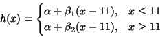
The model called ``Model 1'' in the ANOVA table has regression function

$$h(x) = \gamma + \beta x = \alpha + \beta (x - 11)$$

where $\alpha = \gamma + 11 \beta$. This is obtained by setting $\beta_1 = \beta_2 = \beta$ in the larger model (called ``Model 2'' in the ANOVA table). Hence ``Model 1'' is a submodel of ``Model 2.''

The table gives a P-value P = 0.004277 for the test of model comparison. Since the P-value is very small, this is strong evidence against the small model. Thus we conclude that the piecewise linear model fits and the simple linear model (``Model 1'') doesn't.

Comment

This problem was a learning experience for the teacher. We needed some homework problems like this. It was harder than I thought it would be. Most people had no clear idea of how to show the models were nested. Only two people got full credit.

In order two show the models are nested, you need to show one of two things.

• Every distribution in the little model is also in the big model. Here the models differ only in their regression functions, so you need to show that every regression function in the little model is also in the big model.
• For regression models, we also have the condition that the range of the design matrix for the little model is a subspace of the range of the design matrix for the big model.

These two conditions come to much the same thing (as we shall see below). We can write the regression functions for the little model

$$h(x) = \alpha + \beta x$$

but this is a bad idea given the form of the regression function for the big model

$$h(x) = \begin{cases} \alpha + \beta_1 (x - 11), & x \le 11 \\ \alpha + \beta_2 (x - 11), & x \ge 11 \end{cases}$$ (1)

Because the two $\alpha$'s are not the same. Better to chose another letter (or at least an embellished alpha) for the intercept in the little model

$$h(x) = \gamma + \beta x$$ (2)

Now the question to be answered is what values of $\alpha$, $\beta_1$ and $\beta_2$ in (1) give (2)? It is not enough to just assert that there are some such values. You have to find them.

A little thought suggests $\beta_1 = \beta_2 = \beta$, which collapses the two cases in (1) to one

$$h(x) = \alpha + \beta (x - 11) = (\alpha - 11 \beta) + \beta x,$$ (3)

but the result still doesn't exactly match (2). You still have to remark about chosing $\alpha - 11 \beta = \gamma$, or what is the same, $\alpha = \gamma + 11 \beta$.

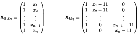
The design matrices for the two models are

$$\mathbf{X}_{\text{little}} = \begin{pmatrix} 1 & x_1 \\ ... ...1 & 0 & x_{n - 1} - 11 \\ 1 & 0 & x_n - 11 \\ \end{pmatrix}$$

How does one show that the range $\mathbf{X}_{\text{little}}$is a subspace of the range of $\mathbf{X}_{\text{big}}$? One needs to show that for any two-vector $\boldsymbol{\beta}_{\text{little}}$, there exists a three-vector $\boldsymbol{\beta}_{\text{big}}$ such that

$$\mathbf{X}_{\text{little}} \boldsymbol{\beta}_{\text{little}} = \mathbf{X}_{\text{big}} \boldsymbol{\beta}_{\text{big}}$$

But this is exactly the same question as asked and answered above, because $\mathbf{X} \boldsymbol{\beta}$ is the regression function described in matrix language. Exactly the same argument shows that

$$\boldsymbol{\beta}_{\text{little}} = (\alpha, \beta)$$

and

$$\boldsymbol{\beta}_{\text{big}} = (\alpha - 11 \beta, \beta, \beta)$$

does the job.

Problem 6

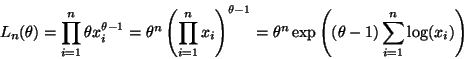
The density of the data is

$$f(x \mid \theta) = \frac{\Gamma(\theta + 1)}{\Gamma(\theta)... ...)} x^{\theta - 1} = \theta x^{\theta - 1}, \qquad 0 < x < 1$$

The prior density is

$$g(\theta \mid \alpha, \lambda) = \frac{\lambda^\alpha}{\Gam... ... \theta^{\alpha - 1} e^{- \lambda \theta}, \qquad \theta > 0$$

(the normalizing constant doesn't matter).

The likelihood for a sample of size n is

$$L_n(\theta) = \prod_{i = 1}^n \theta x_i^{\theta - 1} = \... ...eta^n \exp\left( (\theta - 1) \sum_{i = 1}^n \log(x_i) \right)$$

or, if we introduce the variables $y_i = \log(x_i)$,

$$L_n(\theta) = \theta^n e^{(\theta - 1) n \bar{y}_n} = \theta^n e^{\theta n \bar{y}_n} e^{- n \bar{y}_n}$$

The last term can be dropped, since it does not contain the parameter, giving

$$L_n(\theta) = \theta^n e^{\theta n \bar{y}_n}$$

The unnormalized posterior (likelihood times prior) is

$$\theta^n e^{\theta n \bar{y}_n} \theta^{\alpha - 1} e^{- \la... ... \theta^{n + \alpha - 1} e^{- (\lambda - n \bar{y}_n) \theta}$$

This is clearly proportional to a $\GammaDis(\alpha + n, \lambda - n \bar{y}_n)$. So that is the posterior density.

Sanity Check: Does this make sense? Are both parameters of the posterior positive? Clearly $\alpha + n$ is positive, because we need $\alpha > 0$ for the prior to make sense. How about $\lambda - n \bar{y}_n$? At first sight this doesn't look positive. We need $\lambda > 0$ for the prior to make sense, but how do we know that the other bit doesn't make it negative? Have to think a bit. 0 < x_i < 1, so $y_i = \log(x_i) < 0$ (logs of numbers less than one are negative), so $- \bar{y}_n$ is actually positive despite its appearance, and everything is o. k.

Problem 7

The regression coefficient in question is -0.011464 and R gives its standard error as 0.007784 and the degrees of freedom for error as 17. We only need to look up the t critical value from Table IIIb in Lindgren, which for 90% confidence is 1.74 (note not in the column headed 90, but in the next one over that has 1.645 as the appropriate z critical value at the bottom).

Thus the interval is

$$-0.011464 \pm 1.74 \cdot 0.007784$$

or

$$-0.011464 \pm 0.01354416$$

or

(-0.02500816, 0.0020801)

Problem 8

The sample median $\widetilde{X}_n$ is asymptotically normal center m the population median and variance 1 / 4 n f(m)² (Corollary 2.28 in the notes). Here the population median is zero by symmetry and $f(0) = 2 / \pi$. Hence

$$\widetilde{X}_n \approx \NormalDis\left(0, \frac{\pi^2}{16 n} \right)$$