Stat 5102 (Geyer) Midterm 2

Problem 1

(a)

The likelihood is

$$L_n(p) = \prod_{i = 1}^n p^m (1 - p)^{x_i} = p^{m n} (1 - p)^{\sum_i x_i} = p^{m n} (1 - p)^{n \bar{x}_n}$$

and the log likelihood is

$$l_n(p) = m n \log(p) + n \bar{x}_n \log(1 - p)$$

The derivatives are
$$\begin{align*}l_n'(p) & = \frac{m n}{p} - \frac{n \bar{x}_n}{1 - p} \\ l_n''(p) & = - \frac{m n}{p^2} - \frac{n \bar{x}_n}{(1 - p)^2} \end{align*}$$
Since the second derivative is negative for all p, the log likelihood is a strictly concave and there is at most one local maximum, which is the MLE and the point where the first derivative is zero, if such a point exists. Setting the first derivative to zero and solving for pgives

$$\hat{p}_n = \frac{m}{m + \bar{x}_n}$$

(b)

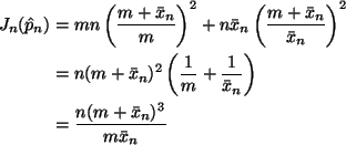
The observed Fisher information is just - l_n''(p)

$$J_n(p) = \frac{m n}{p^2} + \frac{n \bar{x}_n}{(1 - p)^2}$$

This is much simpler than calculating expectations or variances.

(c)

The asymptotic confidence interval using observed Fisher information is

$$\hat{p}_n \pm 1.96 \frac{1}{\sqrt{J_n(\hat{p}_n)}}$$

If you want to simplify that
$$\begin{align*}J_n(\hat{p}_n) & = m n \left(\frac{m + \bar{x}_n}{m} \right)^2 ... ...bar{x}_n}\right) \\ & = \frac{n (m + \bar{x}_n)^3}{m \bar{x}_n} \end{align*}$$
However, that is not necessary for full credit.

Alternate Solutions to Part (b)

Calculating expected Fisher information in part (b) is not advisable unless you recognize that the distribution of the X_i is related to a negative binomial distribution. In fact

$$m + X_i \sim \NegBinDis(m, p)$$

So we can look up (equation (7) on p. 156 in Lindgren)
$$\begin{align*}E(m + X_i) & = \frac{m}{p} \\ \var(m + X_i) & = \frac{m (1 - p)}{p^2} \end{align*}$$
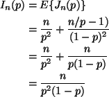
which can be used to calculate expected Fisher information by either method (variance of the first derivative of log likelihood or minus the expectation of the second derivative).

We'll just do the second here

$$E(X{\mkern -13.5 mu}\overline{\phantom{\text{X}}}_n) = E(X_i) = \left(\frac{m}{p} - m\right) = \frac{m (1 - p)}{p}$$

So

$$I_n(p) = E\{J_n(p)\} = \frac{m n}{p^2} + \frac{n m (1 - p)}{p (1 - p)^2} = \frac{n m}{p^2 (1 - p)}$$

When we evaluate at the MLE, we actually get the same thing as with observed Fisher information, that is, $I_n(\hat{p}_n) = J_n(\hat{p}_n)$.

Problem 2

(a)

The likelihood is

$$L_n(\theta) = \prod_{i = 1}^n \theta x_i^{- \theta - 1} = ... ...}^n x_i \right)^{- \theta - 1} = \theta^n a_n^{- \theta - 1}$$

where to simplify notation we have defined the statistic

$$a_n = \prod_{i = 1}^n x_i.$$

The prior is

$$g(\theta) = \lambda e^{- \theta \lambda}$$

so likelihood times prior is

$$\theta^n a_n^{- \theta - 1} \lambda e^{- \theta \lambda} = ... ...\frac{\lambda}{a_n} \theta^n e^{- (\lambda + \log a_n) \theta}$$

which (considered as a function of $\theta$) is an unnormalized $\GammaDis(n + 1, \lambda + \log a_n)$ density. Thus that's the posterior.

$$\theta \mid x_1, \ldots, x_n \sim \GammaDis(n + 1, \lambda + \log a_n)$$

(b)

The mean of a gamma is the shape parameter divided by the scale parameter

$$E(\theta \mid x_1, \ldots, x_n) = \frac{n + 1}{\lambda + \log a_n}$$

Problem 3

(a)

This is a job for Corollary 4.10 in the notes. The inverse transformation is

$$\theta = h(\varphi) = e^\varphi$$

which has derivative

$$h'(\varphi) = e^\varphi$$

Thus the Fisher information for $\varphi$ is

$$\widetilde{I}_1(\varphi) = I_1[h(\varphi)] \cdot [h'(\varph... ...\varphi)^2}{2} \cdot [e^\varphi]^2 = \frac{e^{4 \varphi}}{2}$$

(b)

$$\sqrt{n} (\hat{\varphi}_n - \varphi) \stackrel{\mathcal{D}}{... ...rightarrow} \NormalDis\left(0, \frac{2}{e^{4 \varphi}}\right)$$

or if you prefer

$$\hat{\varphi}_n \approx \NormalDis \left(\varphi, \frac{2}{n e^{4 \varphi}}\right)$$

where, of course $\varphi = \log(\theta)$ is the true parameter value.

Comment.

Part (b) could also be done using the delta method, but that wouldn't reuse part (a).

Problem 4

An exact test is based on the pivotal quantity

$$\frac{(n - 1) S_n^2}{\sigma^2} \sim \ChiSqDis(n - 1)$$

To make a test statistic, we plug in the parameter value hypothesized under the null hypothesis $\sigma^2 = 1$ giving a test statistic T = 9 * 2.3 / 1 = 20.7.

The P-value is P(Y > 20.7) where $Y \sim \ChiSqDis(n - 1)$. From Table Va in Lindgren, this is between 0.014 and 0.015, say P = 0.015. (R says P = 0.014.) Since P < 0.05 the null hypothesis is rejected at the 0.05 level of significance.

Problem 5

The easiest asymptotic test is based on the asymptotically pivotal quantity

$$Z = \frac{X{\mkern -13.5 mu}\overline{\phantom{\text{X}}}_n - \mu}{\sigma / \sqrt{n}}$$

which is approximately standard normal for large n. To do the test in this particular problem we need to plug in the mean and standard deviation of the geometric distribution (from pp. 154-155 in Lindgren)
$$\begin{align*}\mu & = \frac{1}{p} \\ \sigma^2 & = \frac{1 - p}{p^2} \end{align*}$$
So under H₀
$$\begin{align*}\mu & = 4 \\ \sigma^2 & = 12 \end{align*}$$
giving a value of

$$Z = \frac{3.6 - 4}{\sqrt{12 / 100}} = -1.1547$$

The one-tailed P-value is P(Z < -1.1547) where Z is standard normal. From Table I in Lindgren, this is between 0.1251 and 0.1230, say P = 0.124. Of course, here we are doing a two-tailed test, for which the P-value is twice this P = 0.248. Since P > .05 we accept H₀ at the 0.05 level of significance.

Alternate Solution

This was not intended as a likelihood inference problem, but you can make it one. The likelihood is

$$L_n(p) = \prod_{i = 1} p (1 - p)^{x_i - 1} = p^n (1 - p)^{n \bar{x}_n - n}$$

and the log likelihood is

$$l_n(p) = n \log(p) + n (\bar{x}_n - 1) \log(1 - p)$$

with derivatives
$$\begin{align*}l_n'(p) & = \frac{n}{p} - \frac{n (\bar{x}_n - 1)}{1 - p} \\ l_n''(p) & = - \frac{n}{p^2} - \frac{n (\bar{x}_n - 1)}{(1 - p)^2} \end{align*}$$
Since the second derivative is negative for all p, the log likelihood is a strictly concave and there is at most one local maximum, which is the MLE and the point where the first derivative is zero, if such a point exists. Setting the first derivative to zero and solving for pgives

$$\hat{p}_n = \frac{1}{\bar{x}_n}$$

The observed Fisher information is

$$J_n(p) = - l_n''(p) = \frac{n}{p^2} + \frac{n (\bar{x}_n - 1)}{(1 - p)^2}$$

Since $E(X{\mkern -13.5 mu}\overline{\phantom{\text{X}}}_n) = E(X_i) = 1 / p$, the expected Fisher information is
$$\begin{align*}I_n(p) & = E\{J_n(p)\} \\ & = \frac{n}{p^2} + \frac{n / p - ... ...frac{n}{p^2} + \frac{n}{p (1 - p)} \\ & = \frac{n}{p^2 (1 - p)} \end{align*}$$
Although these look a bit different, they are the same when evaluated at the MLE

$$J_n(\hat{p}_n) = I_n(\hat{p}_n) = \frac{n \bar{x}_n^3}{\bar{x}_n - 1}$$

The asymptotically pivotal quantity we use to make a test is

$$Z = (\hat{p}_n - p) \sqrt{I_n(\hat{p}_n)}$$

which is approximately standard normal for large n. Here is
$$\begin{align*}\hat{p}_n & = \frac{1}{3.6} = 0.277778 \\ I_n(\hat{p}_n) & = \fr... ...6 - 1} = 1794.46 \\ Z = (0.277778 - 0.25) \sqrt{1794.46} = 1.1767 \end{align*}$$
Almost the same Z as in the simpler method (the two procedures are asymptotically equivalent). The two-tailed P-value is P = 0.2394 and again H₀ is accepted at the 0.05 level of significance.