Stat 5102 (Geyer) Midterm 1

Problem 1

The basic fact this problem uses is

$$X{\mkern -13.5 mu}\overline{\phantom{\text{X}}}_n \sim \NormalDis\left(\mu, \frac{\sigma^2}{n}\right)$$

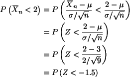
(Theorem 9 of Chapter 7 in Lindgren). To use the normal distribution table in Lindgren we must standardize $X{\mkern -13.5 mu}\overline{\phantom{\text{X}}}_n$
$$\begin{align*}P\left(X{\mkern -13.5 mu}\overline{\phantom{\text{X}}}_n < 2\right... ...ac{2 - 3}{2 / \sqrt{9}} \right) \\ & = P\left(Z < - 1.5 \right) \end{align*}$$
where Z is standard normal (note $\sigma^2 = 4$ so $\sigma = 2$). From Table I in Lindgren

P(Z < - 1.5) = 0.0668.

Problem 2

To use the method of moments, we first need to find some moments. Since this is not a ``brand name'' distribution, we must integrate to find the moments. The obvious moment to try first is the first moment (the mean)
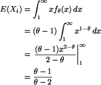
$$\begin{align*}E(X_i) & = \int_1^\infty x f_\theta(x) \, d x \\ & = (\theta... ...eta} \right\vert _1^\infty \\ & = \frac{\theta - 1}{\theta - 2} \end{align*}$$
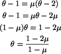
Solving for $\theta$ as a function of $\mu$, we get
$$\begin{gather*}\theta - 1 = \mu (\theta - 2) \\ \theta - 1 = \mu \theta - 2 \m... ... - \mu) \theta = 1 - 2 \mu \\ \theta = \frac{1 - 2 \mu}{1 - \mu} \end{gather*}$$
or perhaps it would be nicer to write

$$\theta = \frac{2 \mu - 1}{\mu - 1}$$

which makes the numerator and denominator both positive. Either way, we get a method of moments estimator by plugging in $X{\mkern -13.5 mu}\overline{\phantom{\text{X}}}_n$for $\mu$

$$\hat{\theta}_n = \frac{2 X{\mkern -13.5 mu}\overline{\phantom... ..._n - 1}{X{\mkern -13.5 mu}\overline{\phantom{\text{X}}}_n - 1}$$

Post Mortem

A lot of students had trouble doing the moment integral. Either they didn't have the pattern clear in their minds

$$\int x^a \, d x = \frac{x^{a + 1}}{a + 1} + \text{const.}$$

(for $a \neq - 1$), or they didn't have the limits of integration right.

Problem 3

This is a symmetric distribution (draw a picture of the density) with center of symmetry $\theta = (a + b) / 2$. Hence $\theta$is both the mean and the median of the population distribution, and both $X{\mkern -13.5 mu}\overline{\phantom{\text{X}}}_n$ and $\widetilde{X}_n$ are consistent and asymptotically normal estimators of $\theta$. So this question makes sense.

(a)

The asymptotic distribution of $X{\mkern -13.5 mu}\overline{\phantom{\text{X}}}_n$ is, as usual, by the CLT,

$$X{\mkern -13.5 mu}\overline{\phantom{\text{X}}}_n \approx \NormalDis\left(\mu, \frac{\sigma^2}{n}\right).$$

Plugging in $\mu = \theta$ and the formula for $\sigma^2$ given by the hint gives

$$X{\mkern -13.5 mu}\overline{\phantom{\text{X}}}_n \approx \NormalDis\left(\theta, \frac{(b - a)^2}{12 n}\right).$$

(b)

The asymptotic distribution of $\widetilde{X}_n$ is, as usual, by Corollary 2.28 in the notes,

$$\widetilde{X}_n \approx \NormalDis\biggl(m, \frac{1}{4 n f(m)^2}\biggr).$$

where m is the population median and f the p. d. f. of the X_i.

By the comments preceeding part (a), $m = \theta$, and by the formula for the density given in the problem statement $f(\theta) = 1 / (b - a)$. Hence

$$\widetilde{X}_n \approx \NormalDis\biggl(\theta, \frac{(b - a)^2}{4 n}\biggr).$$

(c)

The ARE is the ratio of the asymptotic variances, either

$$\frac{(b - a)^2}{12 n} \cdot \frac{4 n}{(b - a)^2} = 3$$

or the the reciprocal 1 / 3, depending on which way you write it.

The better estimator is the one with the smaller asymptotic variance, in this case $X{\mkern -13.5 mu}\overline{\phantom{\text{X}}}_n$.

Post Mortem

Several people got an n in their expression for ARE. This can never happen. ARE is defined as the ratio of asymptotic variances, which do not contain n. If you messed this up, you either forgot an n somewhere or got confused between the two forms of asymptotic expressions. In the mathematically precise forms
$$\begin{align*}\sqrt{n} (S_n - \theta) & \stackrel{\mathcal{D}}{\longrightarrow}\... ...eta) & \stackrel{\mathcal{D}}{\longrightarrow}\NormalDis(0, \tau^2) \end{align*}$$
(this is copied from p. 86 in the notes), the ARE of S_n to T_n is $\sigma^2 / \tau^2$. Note that neither contains an n. No limit of any sort contains an n. In the sloppy forms
$$\begin{align*}S_n & \approx \NormalDis\left(\theta, \frac{\sigma^2}{n} \right) \\ T_n & \approx \NormalDis\left(\theta, \frac{\tau^2}{n} \right) \end{align*}$$
Both variances are proportional to 1 / n and the ratio is $\sigma^2 / \tau^2$ as before, the n's cancel.

Even in the tricky case where one of the estimators does not obey the square root law, e. g., mean versus median for Cauchy or mean versus X_(n) for $\mathcal{U}(0, \theta)$, the ARE still does not contain an n, it would be zero or infinity. An ARE with an n in it is always wrong.

Problem 4

This is a job for Theorem 3.12 in the notes. The problem doesn't specify an equal-tailed interval ( $\beta = \alpha / 2$in the theorem), but that's the most common, so that's what this solution will do. Note that as the comment immediately following the theorem says n V_n = (n - 1) S²_n so we use the theorem with that plugged in.

Our confidence interval for $\sigma^2$ is

$$\frac{(n - 1) S^2_n}{\chi^2_{1 - \alpha / 2}} < \sigma^2 < \frac{(n - 1) S^2_n}{\chi^2_{\alpha / 2}}$$

From Table Vb the two critical values needed are 3.33 and 16.9, giving the interval

$$\frac{9 \cdot 2.2}{16.9} < \sigma^2 < \frac{9 \cdot 2.2}{3.33}$$

or

$$1.17 < \sigma^2 < 5.95$$

Alternate Solutions

Taking $\beta = 0$ or $\beta = \alpha$ in the theorem would give the ``one-tailed'' confidence intervals (0, 4.75) and $(1.35, \infty)$. These are also perfectly acceptable.

Problem 5

This is a problem for the delta method. We know from the properties of the exponential distribution

$$E(X_i) = \frac{1}{\lambda}$$

and

$$\var(X_i) = \frac{1}{\lambda^2}$$

Hence the CLT says in this case

$$X{\mkern -13.5 mu}\overline{\phantom{\text{X}}}_n \approx \NormalDis\left(\frac{1}{\lambda}, \frac{1}{n \lambda^2}\right)$$

For any differentiable function g, the delta method says

$$g(X{\mkern -13.5 mu}\overline{\phantom{\text{X}}}_n) \approx... ...g'\Bigl(\frac{1}{\lambda}\Bigr)^2 \frac{1}{n \lambda^2}\right)$$

The g such that $Y_n = g(X{\mkern -13.5 mu}\overline{\phantom{\text{X}}}_n)$ is

 

g(x) = e^{- t / x} (1)

which has derivative

$$g'(x) = \frac{t}{x^2} e^{- t / x}$$ (2)

so

$$g\Bigl(\frac{1}{\lambda}\Bigr) = e^{- \lambda t}$$

and

$$g'\Bigl(\frac{1}{\lambda}\Bigr) = \lambda^2 t e^{- \lambda t}$$

and

$$Y_n \approx \NormalDis\left(e^{- \lambda t}, \lambda^2 t^2 e^{- 2 \lambda t} / n\right)$$

Post Mortem

Many students got the calculus wrong. They didn't even give themselves a chance to do it right. You can't differentiate a function when you aren't clear what the function is. You must have (1) written down in order to have a chance of producing (2).

Of course the letter x in (1) is a dummy variable. It is perfectly o. k. to write g(u) = e^{- t / u} or $g(\theta) = e^{- t / \theta}$ or the same thing with any other letter substituted for x on both sides of (1). What you can't do is try to differentiate something like

$$g(\theta) = e^{- \lambda t}$$

This doesn't define the function g. So useful as it may be in another part of the problem, it is completely useless for figuring out the derivative $g'(\theta)$.

In order to differentiate a function, you have to know what it is. Write down a correct definition.

Many students got the asymptotic variance wrong for another reason. The got confused between the ``precise'' and ``sloppy'' asymptotic expressions. The univariate delta method says, if

$$\sqrt{n} (T_n - \theta) \stackrel{\mathcal{D}}{\longrightarrow}Y$$

then

$$\sqrt{n} \bigl( g(T_n) - g(\theta) \bigr) \stackrel{\mathcal{D}}{\longrightarrow}g'(\theta) Y$$

(Theorem 1.13 in the notes). The sloppy ``double squiggle'' form is given in the comment after the theorem. If

$$Y \sim \mathcal{N}(0, \sigma^2)$$

then

$$g(T_n) \approx \NormalDis\biggl(g(\theta), \frac{g'(\theta)^2 \sigma^2}{n} \biggr)$$

Note that the variance in the ``double squiggle'' form has $g'(\theta)$squared. This is a consequence of

$$\var(b X) = b^2 \var(X)$$

which in this case implies

$$\var\left\{g'(\theta) Y\right\} = g'(\theta)^2 \var(Y)$$